Simulate the Observation#
To simulate an observation, you require a Target, Instrument,
and a date of observation date_obs.
Warning
jayrock relies on existing services and tools, primarily provided directly
by the STScI. Nevertheless, bugs happen. I strongly recommend to verify the
planning results obtained here with the tools provided by the STScI (JWST GTVT, ETC, APT).
Running the simulation#
The observe function simulates the observation akin to the online
ETC using the STScI’s pandeia python package.
Simulations with pandeia run locally on your machine.
>>> import jayrock

>>> # Target and date_obs
>>> target = jayrock.Target("Ophelia")
>>> target.compute_ephemeris(cycle=6)
>>> date_obs = target.get_date_obs(at="vmag_min")

>>> # Instrument
>>> inst = jayrock.Instrument("MIRI", "MRS")
>>> inst.aperture = 'ch2'
>>> inst.disperser = 'medium'
>>> inst.detector.nexp = 4
>>> inst.detector.ngroup = 10
>>> inst.detector.nint = 1

>>> # Run simulation
>>> obs = jayrock.observe(target, inst, date_obs)
INFO     [jayrock] Observing Target(name=Ophelia) with MIRI|mrs on 2028-03-30
INFO     [jayrock] ch2|medium - ngroup=10|nint=1|nexp=4 - readout=fastr1
INFO     [jayrock] SNR=766.0 at 9.41μm in 1.9min
WARNING  [jayrock] Observation warnings: {'cube_partial': 'There are 352 total
                   partially saturated pixels in the data cube.'}
Inspecting the Report#
The observe function returns an Observation object that contains the
same report as generated by the online ETC.
>>> obs.report.keys()
dict_keys(['sub_reports', 'input', '1d', '2d', '3d', 'scalar', 'information', 'transform', 'warnings', 'web_report'])
>>> obs.report['scalar']['sn']  # snr at reference wavelength
765.9608182878744
>>> wave, snr = obs.report['1d']['sn']  # snr over wavelength
>>> wave[:5]
[8.6909816  8.69261246 8.69424332 8.69587418 8.69750504]
>>> snr[:5]
[648.42203743 648.33386155 648.24524604 648.15622563 648.06695908]
Refer to the pandeia documentation for details on the report structure and available information.
Some frequently used properties are directly accessible from the Observation object.
>>> obs.snr  # snr at reference wavelength
>>> obs.texp  # exposure time in seconds
>>> obs.plot_snr()  # plot snr over wavelength
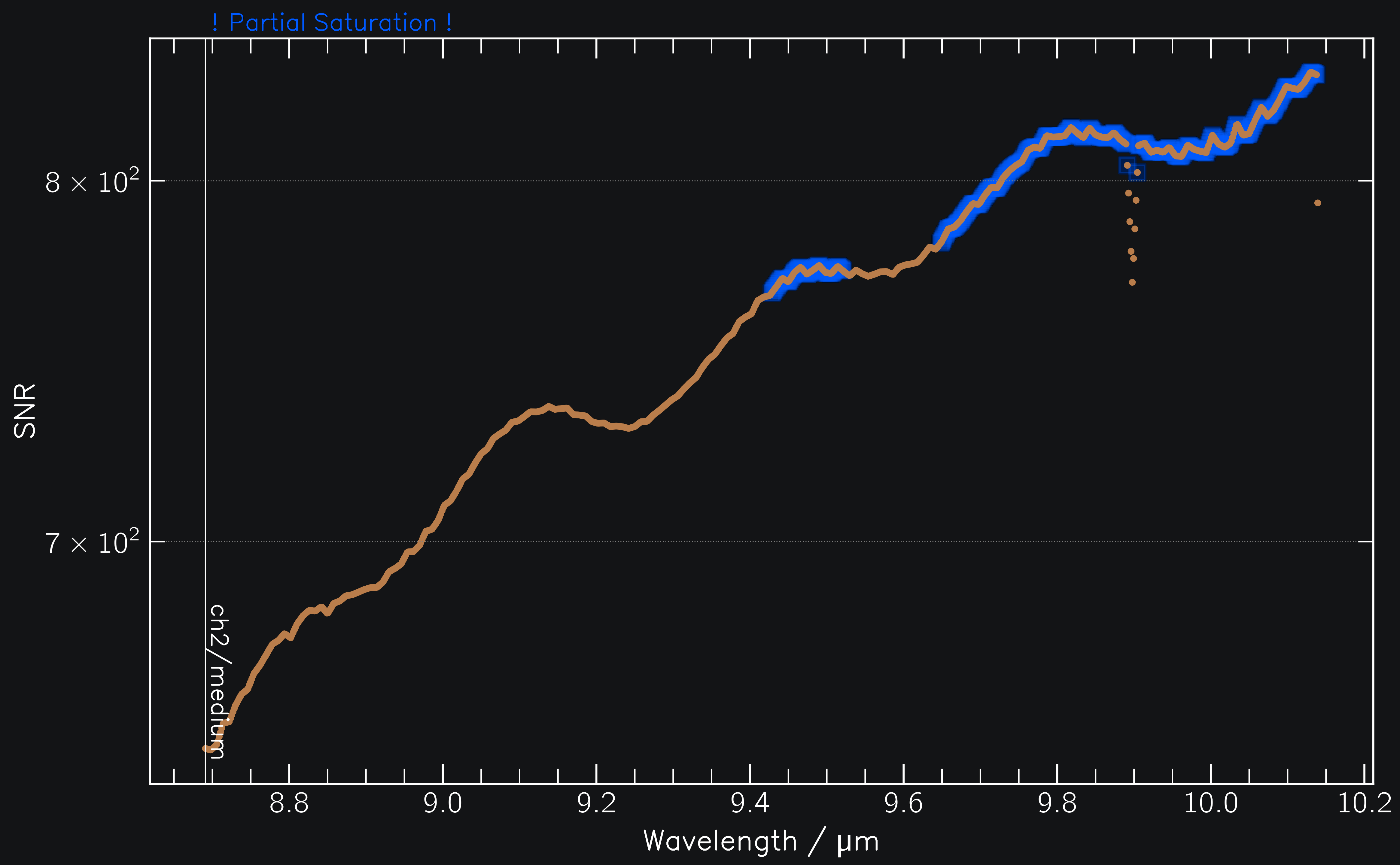
Fig. 1: SNR of MIRI observations of (171) Ophelia.#
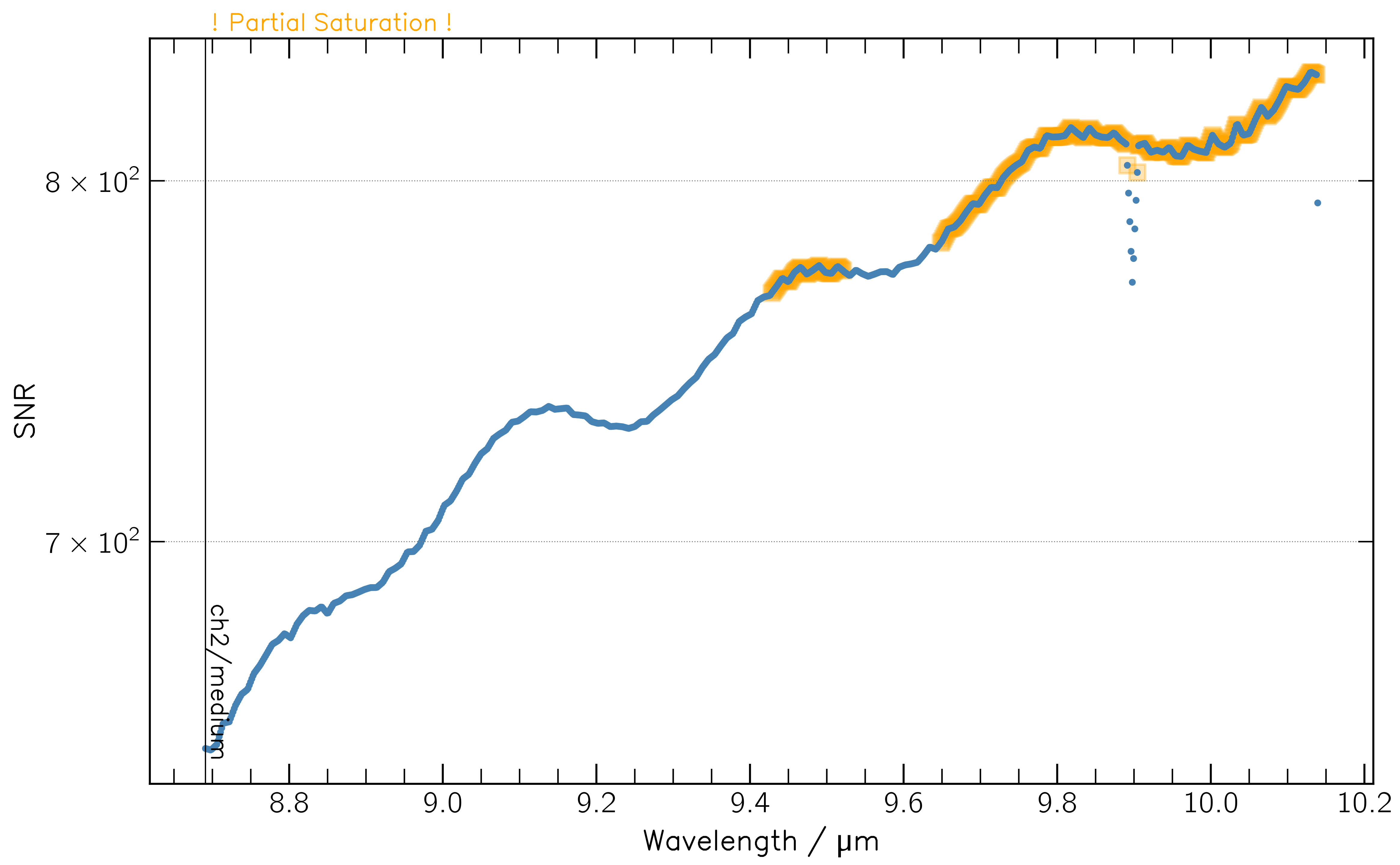
Fig. 1: SNR of MIRI observations of (171) Ophelia.#
Identifying saturation#
If the detector saturates during the observation, this is indicated in multiple ways.
(1) Warnings are written to the console during the simulation via jayrock.observe (see above)
(2) The saturated wavelengths are framed in orange (partial sat.) or purple (full sat.) in the SNR plot.
(3) The report has different attributes to identify saturated pixels:
>>> obs.partially_saturated # boolean array over wavelength. True where partially saturated
array([False, False, False, ...,  True,  True,  True, ..., False, False])

>>> obs.fully_saturated # boolean array over wavelength. True where fully saturated
array([False, False, False, ...,  False,  False,  False, ..., False, False])

>>> obs.n_partial_saturated # number of partially saturated pixels per wavelength
[0, 0, 0, ..., 1, 1, 1, ..., 0, 0]

>>> obs.is_saturated  # any wavelength fully or partially saturated?
True
Observing in multiple configurations#
Each observation uses one specific instrument configuration. To simulate observations of the same target with different configurations, simply use a loop. This is especially useful for MIRI MRS, where each aperture and disperser needs to be simulated separately.
observations = []
for aperture in ['ch1', 'ch2', 'ch3', 'ch4']:
     for disperser in ['short', 'medium', 'long']:
         inst.aperture = aperture
         inst.disperser = disperser
         obs = jayrock.observe(target, inst, date_obs)
         observations.append(obs)
You can then plot the SNRs of all observations together:
>>> jayrock.plot_snr(observations) # plot SNRs of multiple observations together
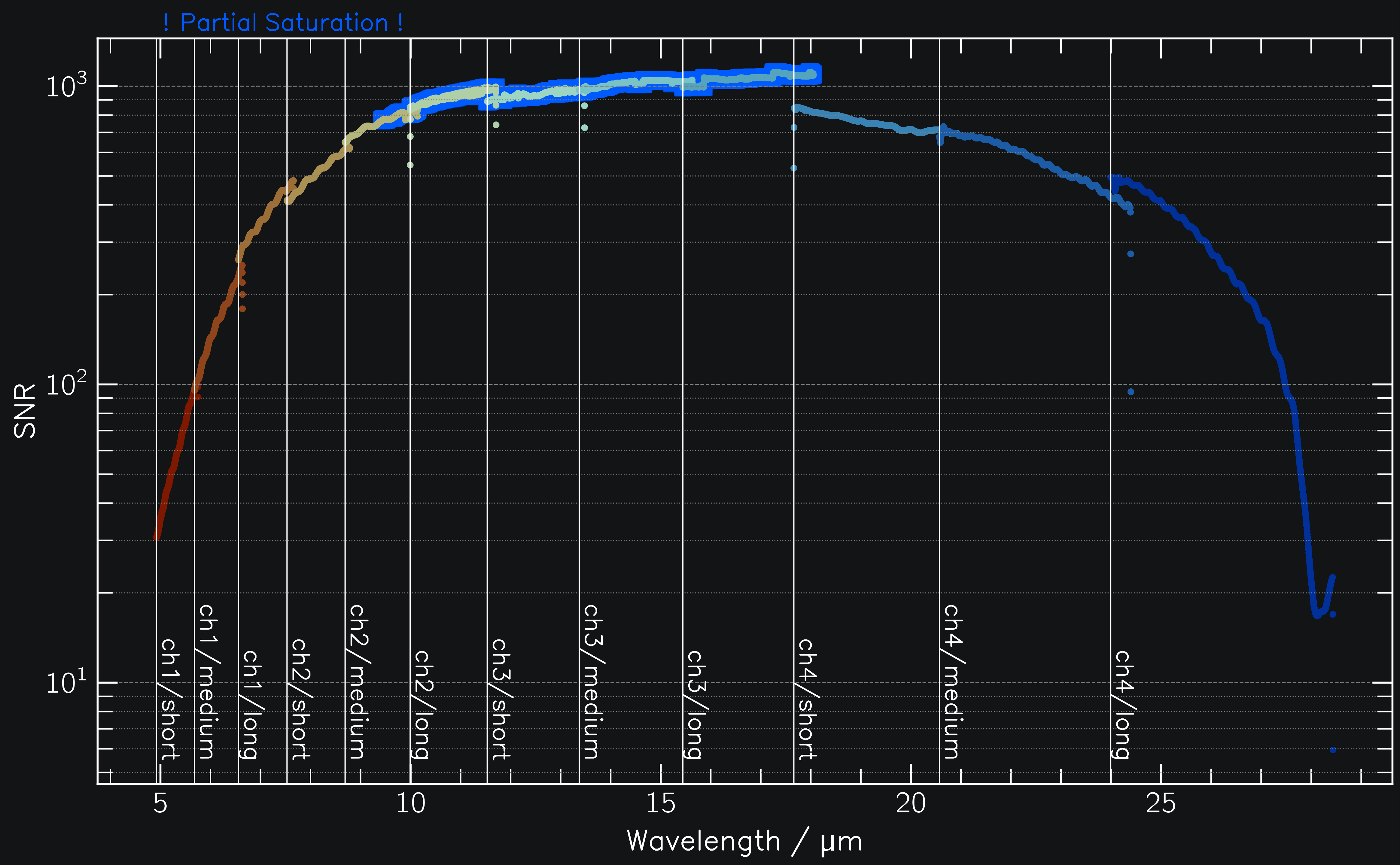
Fig. 2: SNR of MIRI observations of (171) Ophelia across all channel/disperser combinatios.#
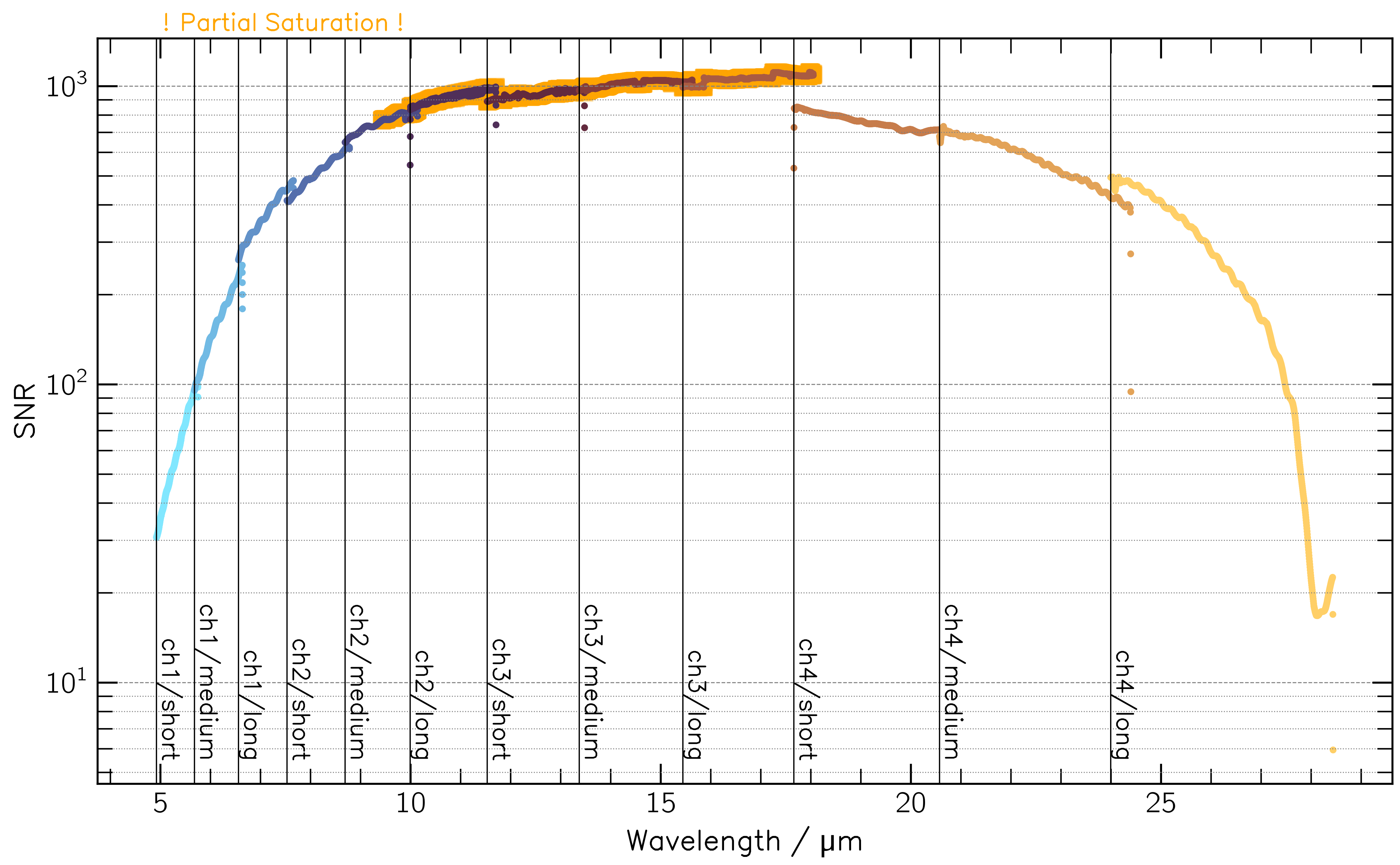
Fig. 2: SNR of MIRI observations of (171) Ophelia across all channel/disperser combinatios.#
Observing on multiple dates#
You might want to compare the SNR obtained at two different epochs, e.g. to optimise the exposure settings for the faintest epoch while ensuring that the observation does not at saturate at the brightest one.
observations = []
date_thermal_min, date_thermal_max = target.get_date_obs(at=["thermal_min", "thermal_max"])
for date_obs in [date_thermal_min, date_thermal_max]:
     obs = jayrock.observe(target, inst, date_obs)
     observations.append(obs)
jayrock.plot_snr(observations)  # plot SNRs of multiple observations together
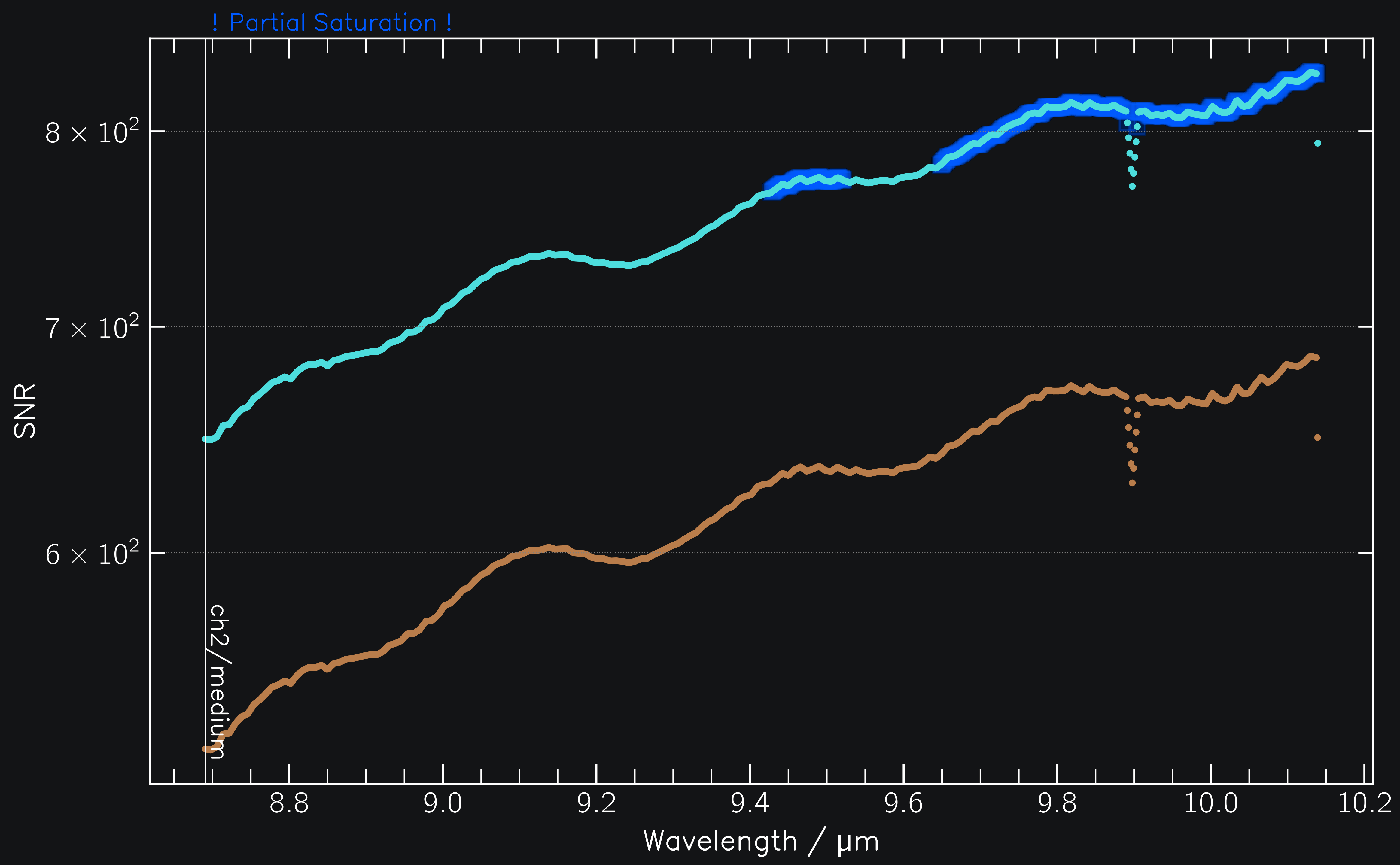
Fig. 3: SNR of MIRI observations of (171) Ophelia at two different dates.#
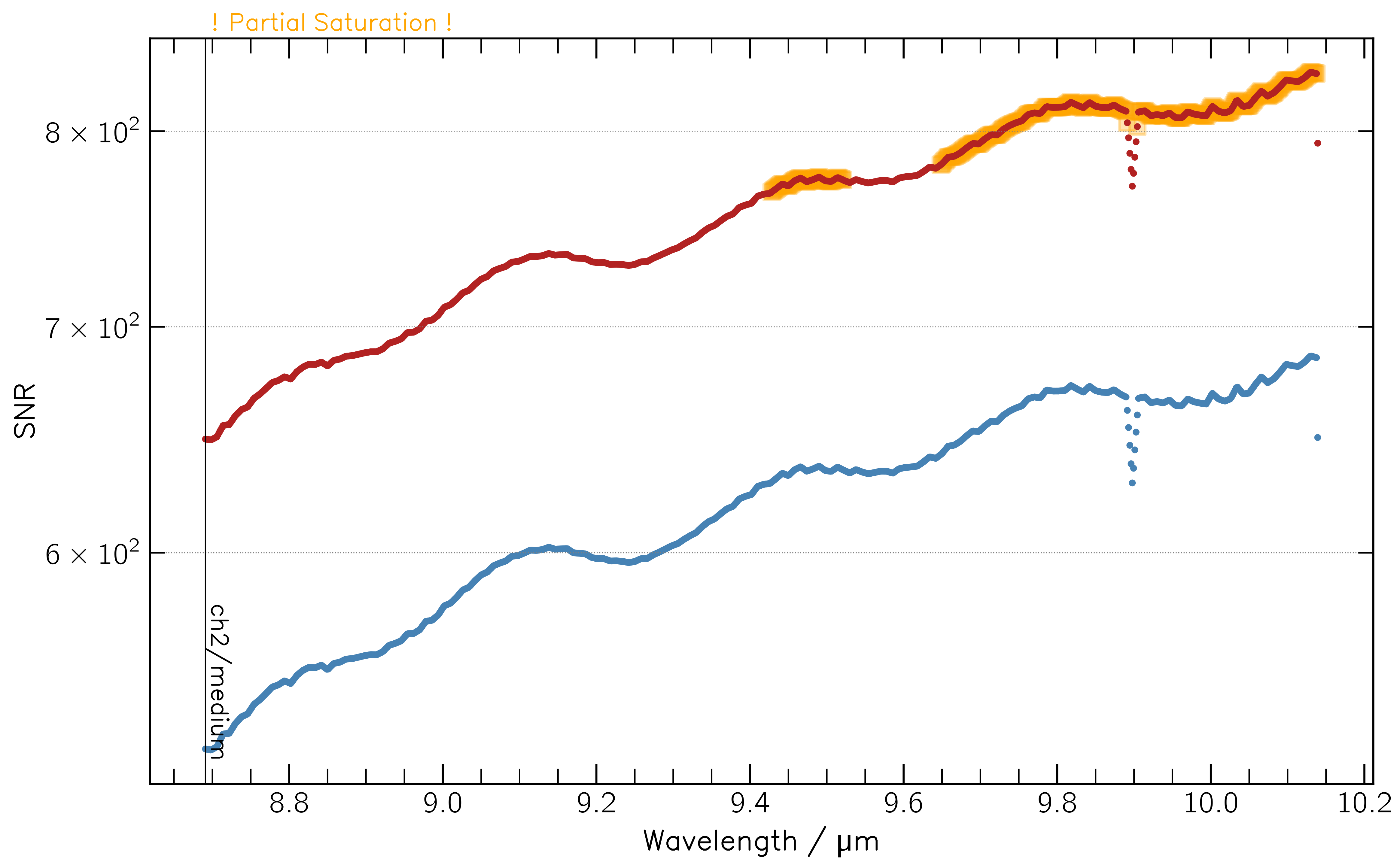
Fig. 3: SNR of MIRI observations of (171) Ophelia at two different dates.#
See the MIRI MRS example for a practical implementation.