Observing TNOs with NIRSpec

After DiSCo comes CoFFEe (Comparison of Fluxes, Feasibility, and Exposure times with NIRSpec):[1] We investigate the observability of hot and cold classicals with NIRSpec IFU and Fixed Slit.

We need the following packages.

from astroquery.jplhorizons import Horizons
from astroquery.mast.missions import MastMissions
from astropy.time import Time
import jayrock
import matplotlib.pyplot as plt
import numpy as np
import pandas as pd
import rocks

Learning from experience: The MAST Archive

Approaching a new telescope, we can learn a lot from previous observing runs. The JWST archive contains the instrumental configuration and target list of previous programmes, which we can query and inspect using the astroquery package. For TNOs, the flagship programme so far is DiSCo-TNOs, programme ID 2418. Let’s query the programmes target list and observation metadata from the MAST archive.

missions = MastMissions(mission="jwst")
disco = missions.query_criteria(program=2418)

# I like pandas DataFrames more than astropy Tables
disco = disco.to_pandas()

This dataframe contains a lot of interesting information:

>>> len(set(disco.targprop))  # how many individual targets were observed?
59
>>> disco.columns.values  # what kind of metadata is in the archive?
['ArchiveFileID' 'fileSetName' 'productLevel' 'targprop' 'targ_ra'
 'targ_dec' 'instrume' 'exp_type' 'opticalElements' 'date_obs' 'duration'
 'program' 'observtn' 'visit' 'publicReleaseDate' 'pi_name'
 'proposal_type' 'proposal_cycle' 'targtype' 'access' 'cal_ver' 'ang_sep'
 's_region']
>>> set(disco.exp_type)  # which instrument/mode combinations?
{'NRS_IFU'}
>>> set(disco.opticalElements) # which disperser/filter combinations?
{'CLEAR;PRISM'}

A common issue in these databases is that minor body names (here in the targprop column) are written in different manners (e.g. 2000ny27, 2000_ny27, 2000 NY27). We use rocks.id to get uniformly formatted designations and numbers.

Less readable but shorter:

names, numbers = zip(*rocks.id(disco.targprop))``

# typo in disco database: sila-nuMaN -> sila-nuNaM
disco.loc[disco.targprop == "SILA-NUMAN", "targprop"] = "SILA-NUNAM"

# add uniform id columns
rock_ids = rocks.id(disco.targprop)  # turns e.g. "1977ub" into ('Chiron', 19521)
names = [name for name, number in rock_ids]
numbers = [number for name, number in rock_ids]

disco['target_name'] = names
disco['target_number'] = numbers

For the purpose of this tutorial, we are most interested in the correlation between exposure time and apparent V magnitude at the time of observation that the DiSCo team chose. We have the date_obs information for each target. We can get the apparent V magnitude from JPL Horizons.

# DiSCo used a 4-point dither - we only want to look at one
# of these observations for each target
disco = disco.drop_duplicates("target_name")

def get_vmag_at_tobs(target, date):
    """Get the V-band magnitude of a target at a specific date via JPL Horizons."""

    # These guys often cause trouble in queries. We ignore them for simplicity.
    if target in ["Gǃkúnǁʼhòmdímà", "ǂKá̦gára"]:
        return np.nan

    # Run the Horizons query
    obj = Horizons(
        id=target, location="500@-170", epochs=Time(date).jd, id_type="asteroid_name"
    )

    # Return V
    return obj.ephemerides()["V"].value[0]

# Query the V mag of the DiSCo targets at the date of their observation
disco["vmag_at_tobs"] = archive.apply(
    lambda row: get_vmag_at_tobs(row["target_name"], row["date_obs"]), axis=1
)

Now we can plot the exposure time versus apparent V magnitude of the DiSCo targets. Note that we multiply the times by four as DiSCo used a 4-point dithering pattern.

fig, ax = plt.subplots()
ax.scatter(disco["vmag_at_tobs"], disco["duration"] / 60 * 4, c="black", marker="v")
ax.set(xlabel="Vmag at time of observation", ylabel="Exposure Duration / min")
fig.savefig("/tmp/disco_vmag_vs_duration.png", backend="pgf")

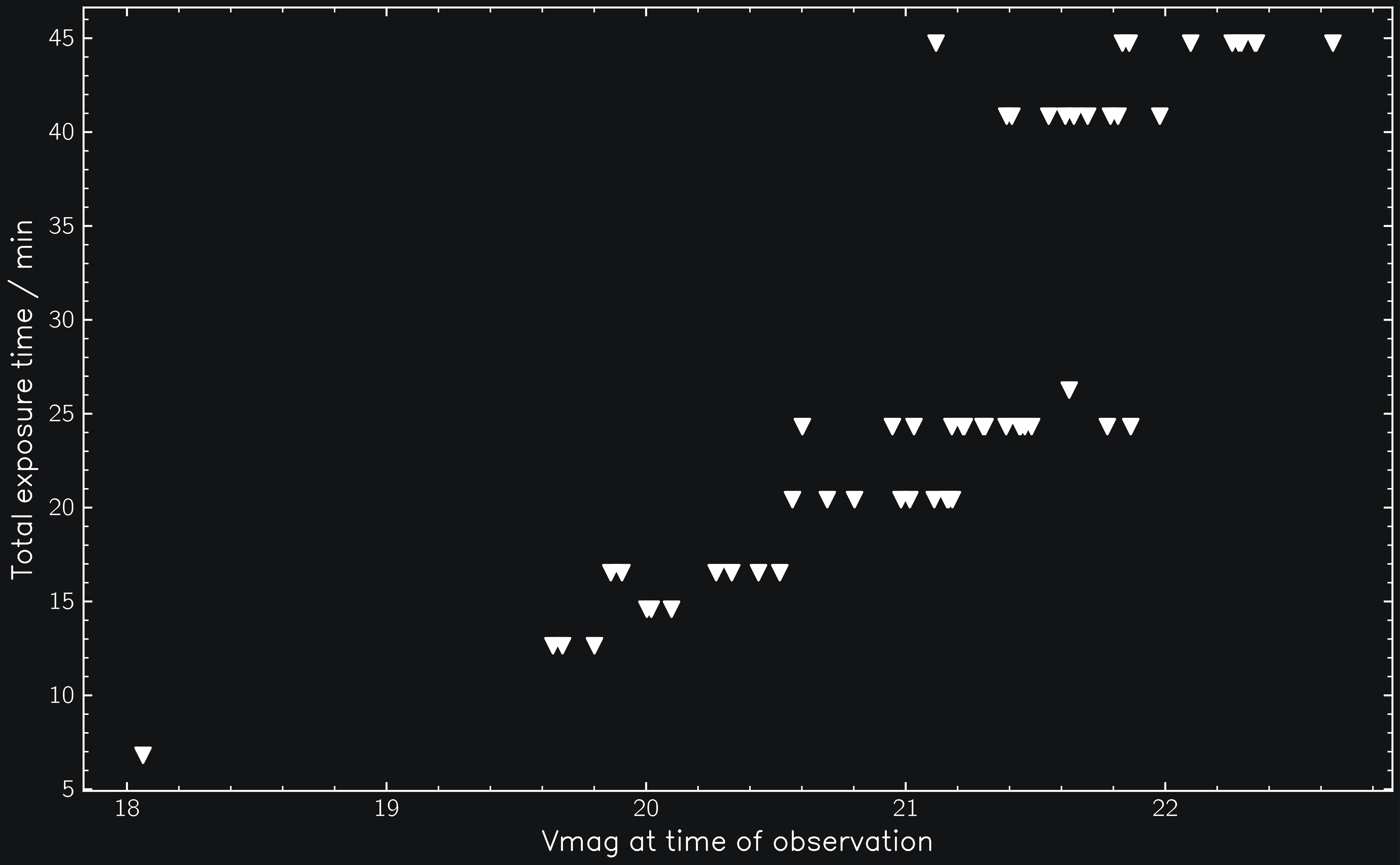
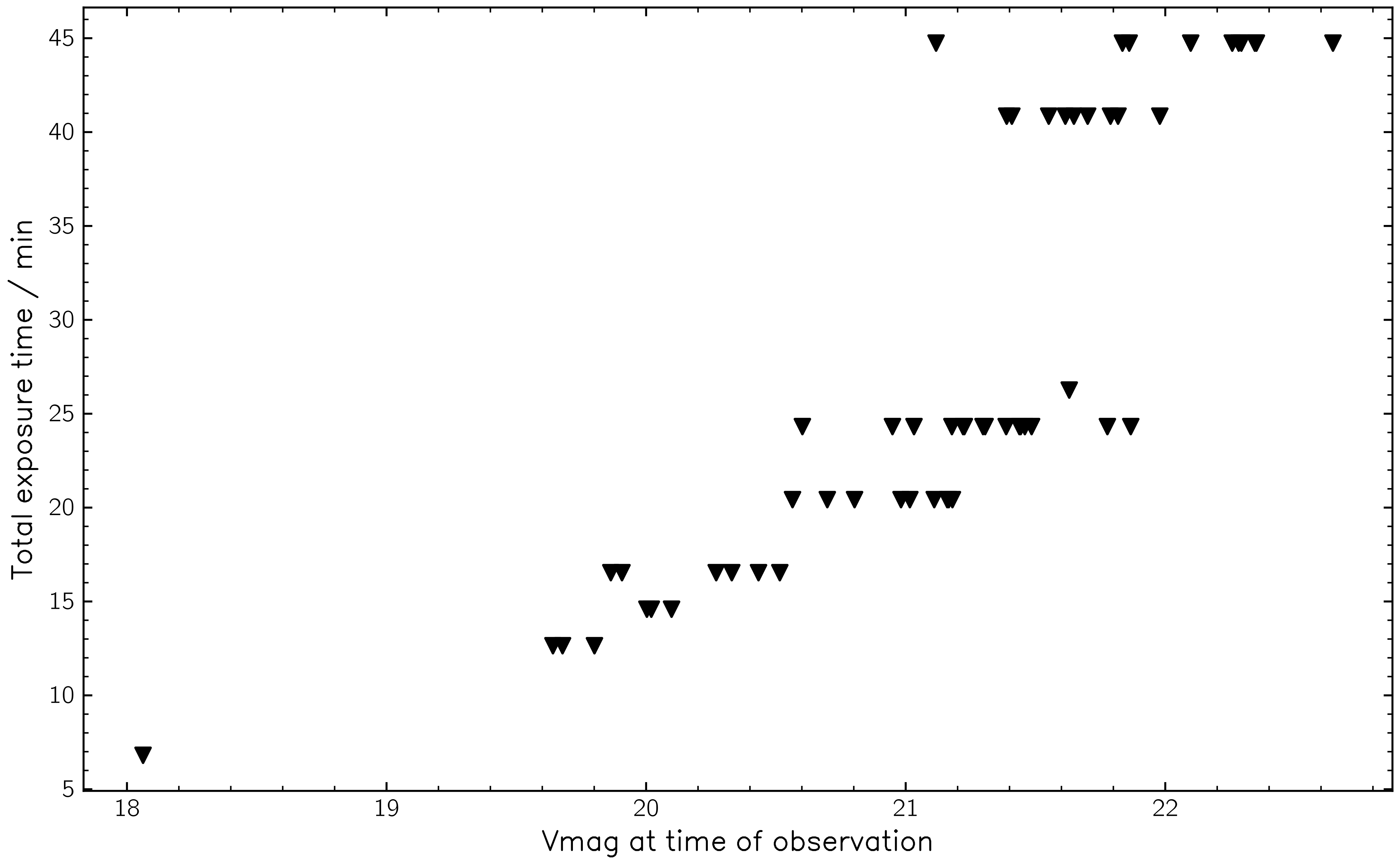
Fig. 1: Apparent V magnitude versus total exposure time for 57 of 59 DisCO targets.

This quick look into the archive thus showed us that DiSCo targeted TNOs up to V~23, with maximum total exposure times of 45 minutes. They used NIRSpec/IFU, a 4-point dithering strategy, and the PRISM/CLEAR disperser/filter combination.

With this information in mind, let’s get to our classicals.

Target selection

List of classicals with rocks

The first thing we need is a list of all known classicals. We use rocks to load the big flat table of minor body properties from SsODNet. This table contains basic properties of all known minor bodies (> 1,400,000). We select classicals based on the pre-defined orbital classes.

all_minor_bodies = rocks.load_bft()

is_classical = all_minor_bodies["sso_class"].str.startswith("KBO>Classical")
classicals = all_minor_bodies[is_classical]

len(classicals) returns 1366 at the time of this writing.

We drop classicals already observed by DiSCo. rocks.id returns the same name/designation as stored in the sso_name column of the BFT, so we can directly compare them.

classicals = classicals[
    ~classicals["sso_name"].isin(disco["target_name"].values)
].reset_index(drop=True)

This removes six classicals, leaving us with 1360 remaining candidates.

Ephemeris query with JPL

Next, we want to know which classicals are visible during JWST cycle 6. We achieve this by looping over our list of classicals and querying their ephemeris from JPL Horizons though jayrock. We add this information to the classicals dataframe.

We use thermal=False in compute_ephemeris to speed up the execution – the NEATM of our targets is not needed here.

for idx, classical in classicals.iterrows():

    # Create target and compute ephemeris with JPL
    target = jayrock.Target(classical["sso_name"])
    target.compute_ephemeris(cycle=6, thermal=False)

    # Record number of days the target is visible by JWST in Cycle 6
    classicals.loc[idx, "n_days_vis"] = len(target.ephemeris)

    # Record the positional uncertainties and distance from the Sun
    date_vmag_min = target.get_date_obs(at="vmag_min")

    ephemeris_on_date_obs = target.ephemeris.loc[
        target.ephemeris.date_obs == date_vmag_min
    ].squeeze()  # just for convenience

    # add all columns from ephemeris_on_date_obs to classicals
    for col in ephemeris_on_date_obs.index:
        classicals.loc[idx, col] = ephemeris_on_date_obs[col]

The JPL Horizons queries may time out and cause the script to fail. In this case, run the queries in smaller batches and combine the results.

This loop ran for about 1.5h on my machine (~4s per target). Time for a coffee break.

Distribution of n_days_vis

Now that we have the ephermis information of our candidate targets, we use different criteria to filter out less practical targets.

First, we check if all targets are visible from JWST during cycle 6.

print(classicals["n_days_vis"].describe())

count    1360.000000
mean      103.133088
std         6.017445
min        99.000000
25%       101.000000
50%       102.000000
75%       103.000000
max       194.000000
Name: n_days_vis, dtype: float64

The minimum number of visible days is 99 days – plenty of time. All candidates pass this stage.

Distribution of \(\sigma_{\textrm{RA}}\) vs \(\sigma_{\textrm{Dec}}\)

Next, we consider whether we can point at a given candidate target. The NIRSpec IFU has a field of view (FoV) of 3”x3”. Orbital uncertainties larger than 1.5” thus mean that the target may not be in the FoV after blind pointing of the telescope to the pre-computed position. We exclude these cases from our list of candidates.

Warning

In practice, we would need to place even stronger constraints due to the dithering offset. We ignore this here.

fig, ax = plt.subplots()

# Plot classicals
ax.scatter(
    classicals["ra_3sigma"], classicals["dec_3sigma"], c="black", alpha=0.5, marker='.'
)

# Add NIRSpec FoV
ax.plot([0, 1.5, 1.5], [1.5, 1.5, 0], color="red", lw=2)

# Add description
ax.text(0.2, 0.05, '1.5"', transform=ax.transAxes, color="red", ha="center")
ax.text(0.12, 0.26, "NIRSpec IFU FoV", transform=ax.transAxes, color="red", ha="center")
ax.text(0.12, 0.29, r"12.2\% of Classicals are within", transform=ax.transAxes, ha="center")

# Final touches
ax.set_xlabel(r"$\sigma_{\textrm{RA}}$ / arcsec")
ax.set_ylabel(r"$\sigma_{Dec}$ / arcsec")
ax.set(xscale="log", yscale="log")
plt.show()

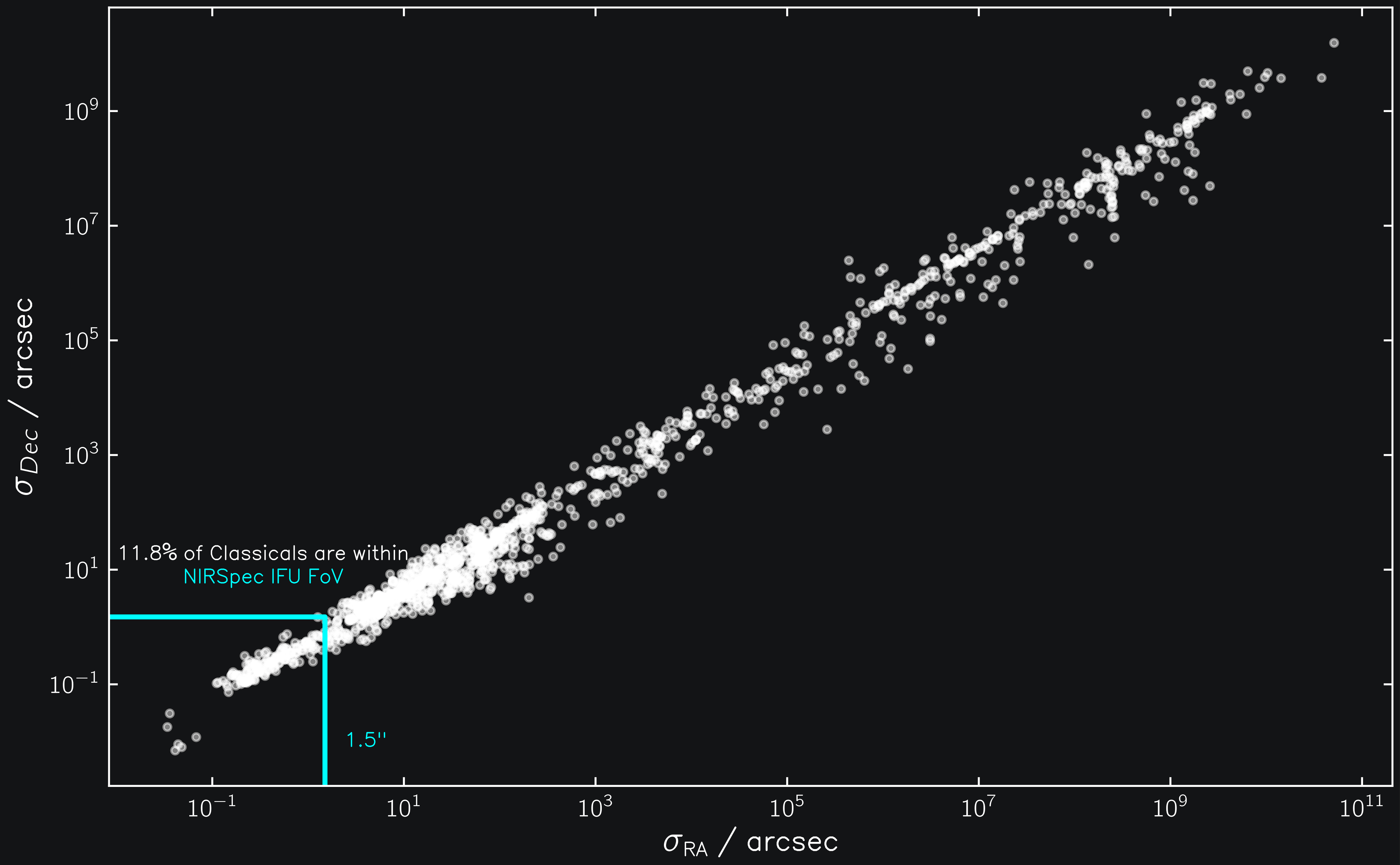
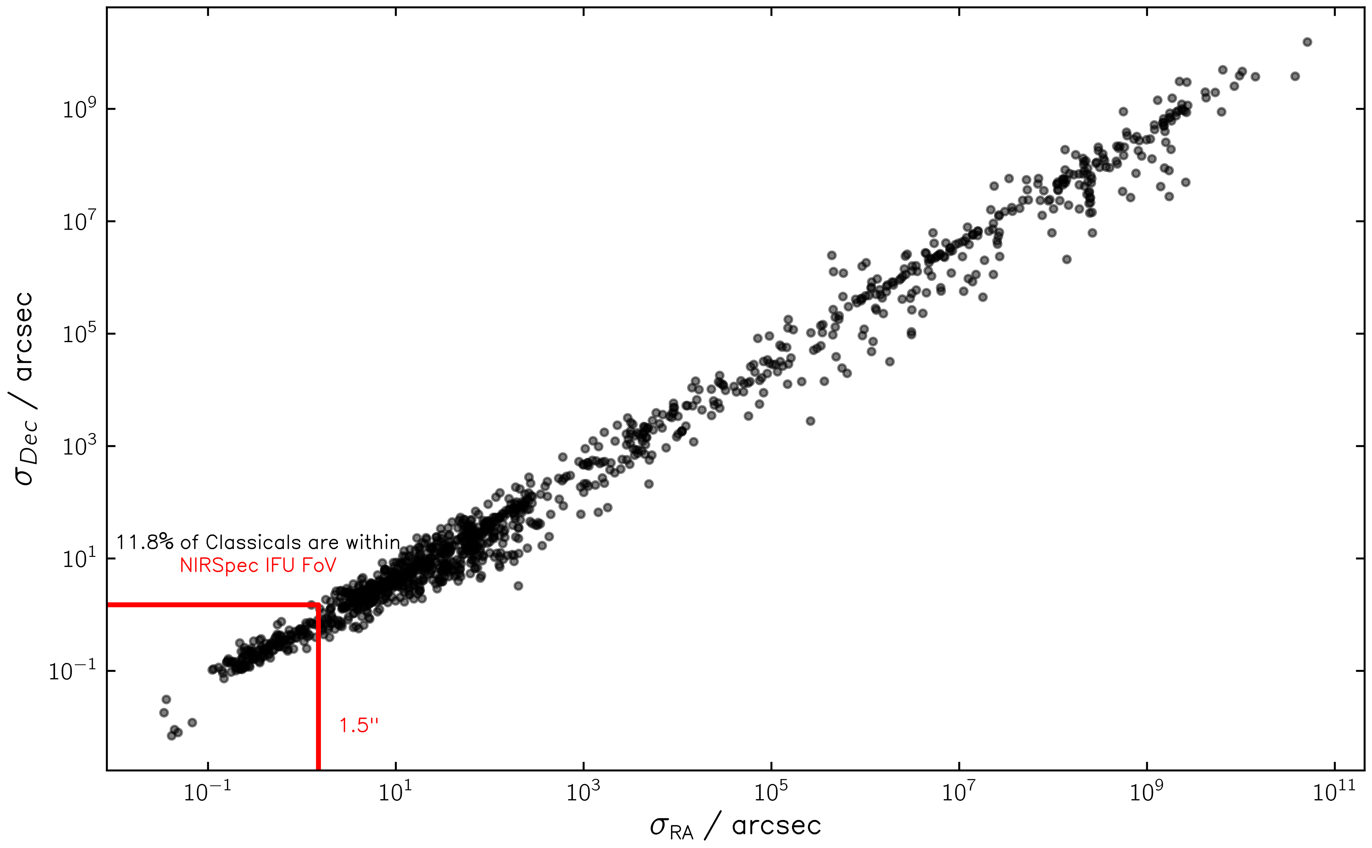
Fig. 2: Positional uncertainty of 1366 cold/hot classicals during JWST Cycle 6.

We reject all candidate targets with orbital uncertainties larger than 1.5” in either RA or Dec.

classicals = classicals[(classicals.ra_3sigma < 1.5) & (classicals.dec_3sigma < 1.5)]

This leaves us with 160 candidate targets.

Distribution of vmag

The filter based on orbital uncertainty removes primarily faint targets. The distribution of the predicted brightest apparent V magnitude of our candidates at the time of observation now looks like this:

print(classicals["vmag"].describe())

count    160.000000
mean      22.167512
std        0.735639
min       18.812000
25%       21.833750
50%       22.278000
75%       22.694000
max       23.714000
Name: vmag, dtype: float64

Following DiSCo, we remove targets with predicted magnitudes larger than 23.

classicals = classicals[classicals.vmag < 23].reset_index(drop=True)

149 candidate targets remain.

NIRSpec configuration

NIRSpec offers two modes suited for our science case here: Fixed Slit and IFU. Fixed Slit offers higher sensitivity at the price of higher overhead costs due to the required slit alignment, while the IFU is less sensitive but is more suited for targets with larger positional uncertainties due to its 3”x3” FoV.

We investigate both modes here. First, we configure them using jayrock.

Fixed Slit

For Fixed Slit observations, we use a 2-point dithering pattern and the recommended nrsirs2rapid readout. Following DiSCo, we use the PRISM/CLEAR disperser/filter combination.

nirspec_fs = jayrock.Instrument("nirspec", "fixed_slit")

nirspec_fs.disperser = "prism"
nirspec_fs.filter = "clear"

nirspec_fs.detector.nexp = 2
nirspec_fs.detector.readout_pattern = "nrsirs2rapid"

IFU

The IFU configuration is similar, only that we employ a 4-point dithering pattern instead.

nirspec_ifu = jayrock.Instrument("nirspec", "ifu")

nirspec_ifu.disperser = "prism"
nirspec_ifu.filter = "clear"

nirspec_ifu.detector.nexp = 4
nirspec_ifu.detector.readout_pattern = "nrsirs2rapid"

SNR versus vmag with IFU

The DiSCo team limited the targets to vmag<23 and the total exposure duration to 45 minutes. Out of curiosity, let’s see how the SNR depends on V. We get the targets that are closest to a given V magnitude in our candidate list and compute the SNR with a fixed instrument configuration, notably 59.3min of total exposure time.

for vmag in [19, 20, 21, 22, 23]:
    tno_closest_in_vmag = classicals.iloc[
        (classicals["vmag"] - vmag).abs().argsort()[:1]
    ].squeeze()

    # Simulate NIRSpec observation
    target = jayrock.Target(tno_closest_in_vmag["sso_name"])
    target.compute_ephemeris(cycle=6)

    # set larger nint/ngroup
    nirspec_ifu.detector.nint = 1
    nirspec_ifu.detector.ngroup = 60

    date_obs = target.get_date_obs(at="vmag_min")
    obs = jayrock.observe(target, nirspec_ifu, date_obs)

This yields the following output:

As the warning tells us, jayrock could not find a literature albedo or diameter for 2014 DN143 and uses default values instead. We do not care about this here as the thermal flux will be negligible either way. However, for targets closer to the Sun / JWST, this could be relevant, and you should set sensible values manually.

Quaoar 18.812  # closest to Vmag 19
INFO     [jayrock] Observing Target(name=Quaoar) with NIRSpec|ifu on 2028-05-22
INFO     [jayrock] prism|clear - ngroup=60|nint=1|nexp=4 - readout=nrsirs2rapid
INFO     [jayrock] SNR=275.1 at 2.95μm in 59.3min
WARNING  [jayrock] Observation warnings: {'cube_partial': 'There are 121 total partially saturated pixels
         in the data cube.'}

2002 TX300 20.011  # closest to Vmag 20
INFO     [jayrock] Observing Target(name=2002 TX300) with NIRSpec|ifu on 2027-10-02
INFO     [jayrock] prism|clear - ngroup=60|nint=1|nexp=4 - readout=nrsirs2rapid
INFO     [jayrock] SNR=153.9 at 2.95μm in 59.3min

Chaos 20.877  # closest to Vmag 21
INFO     [jayrock] Observing Target(name=Chaos) with NIRSpec|ifu on 2027-11-17
INFO     [jayrock] prism|clear - ngroup=60|nint=1|nexp=4 - readout=nrsirs2rapid
INFO     [jayrock] SNR=96.2 at 2.95μm in 59.3min

2014 DN143 22.003  # closest to Vmag 22
WARNING  [jayrock] No albedo value on record for 2014 DN143. Using default of 0.1.
WARNING  [jayrock] No diameter value on record for 2014 DN143. Using default of 30km.
INFO     [jayrock] Observing Target(name=2014 DN143) with NIRSpec|ifu on 2028-02-15
INFO     [jayrock] prism|clear - ngroup=60|nint=1|nexp=4 - readout=nrsirs2rapid
INFO     [jayrock] SNR=47.5 at 2.95μm in 59.3min

2001 QC298 22.964  # closest to Vmag 23
INFO     [jayrock] Observing Target(name=2001 QC298) with NIRSpec|ifu on 2027-08-25
INFO     [jayrock] prism|clear - ngroup=60|nint=1|nexp=4 - readout=nrsirs2rapid
INFO     [jayrock] SNR=23.4 at 2.95μm in 59.3min

Asteroids fainter than vmag 23 will have SNRs smaller than ~20 within 60minute exposure time. The cut-off at 23 thus seems reasonable.

Estimating SNR and defining exposure times

We know that Fixed Slit and IFU have different sensitivities. How does this translate into exposure times and SNR? For our candidate list of 160 targets, we compute the required exposure time to reach an SNR of 40-50 at 3μm. We provide this range instead of a fixed value to speed up the binary search for the best ngroup/nint settings.

for idx, classical in classicals.iterrows():

    # Create target and compute ephemeris with JPL
    target = jayrock.Target(classical["sso_name"])
    target.compute_ephemeris(cycle=6)

    date_obs = target.get_date_obs(at="vmag_min")

    # Compute SNR parameters for IFU and Fixed Slit
    for inst in [nirspec_ifu, nirspec_fs]:
        inst.set_snr_target([40,50], target, date_obs, wave=3)

        classicals.loc[idx, f"{inst.mode}_nint"] = inst.detector.nint
        classicals.loc[idx, f"{inst.mode}_ngroup"] = inst.detector.ngroup
        classicals.loc[idx, f"{inst.mode}_texp"] = inst.texp
        classicals.loc[idx, f"{inst.mode}_snr"] = inst.estimated_snr

This takes a while – another coffee break is recommended.

After completion, we compare the required exposure time against apparent V magnitude for the two modes.

fig, ax = plt.subplots()
ax.scatter(
    classicals["vmag"],
    classicals["fixed_slit_texp"] / 60,
    c="black",
    marker=".",
    alpha=1,
    label="NIRSpec Fixed Slit",
)
ax.scatter(
    classicals["vmag"],
    classicals["ifu_texp"] / 60,
    c="orange",
    marker="x",
    alpha=0.7,
    label="NIRSpec IFU",
)
ax.set(
    xlabel="Vmag at time of observation",
    ylabel="Total exposure time / min",
    yscale="log",
)
ax.legend()
plt.show()

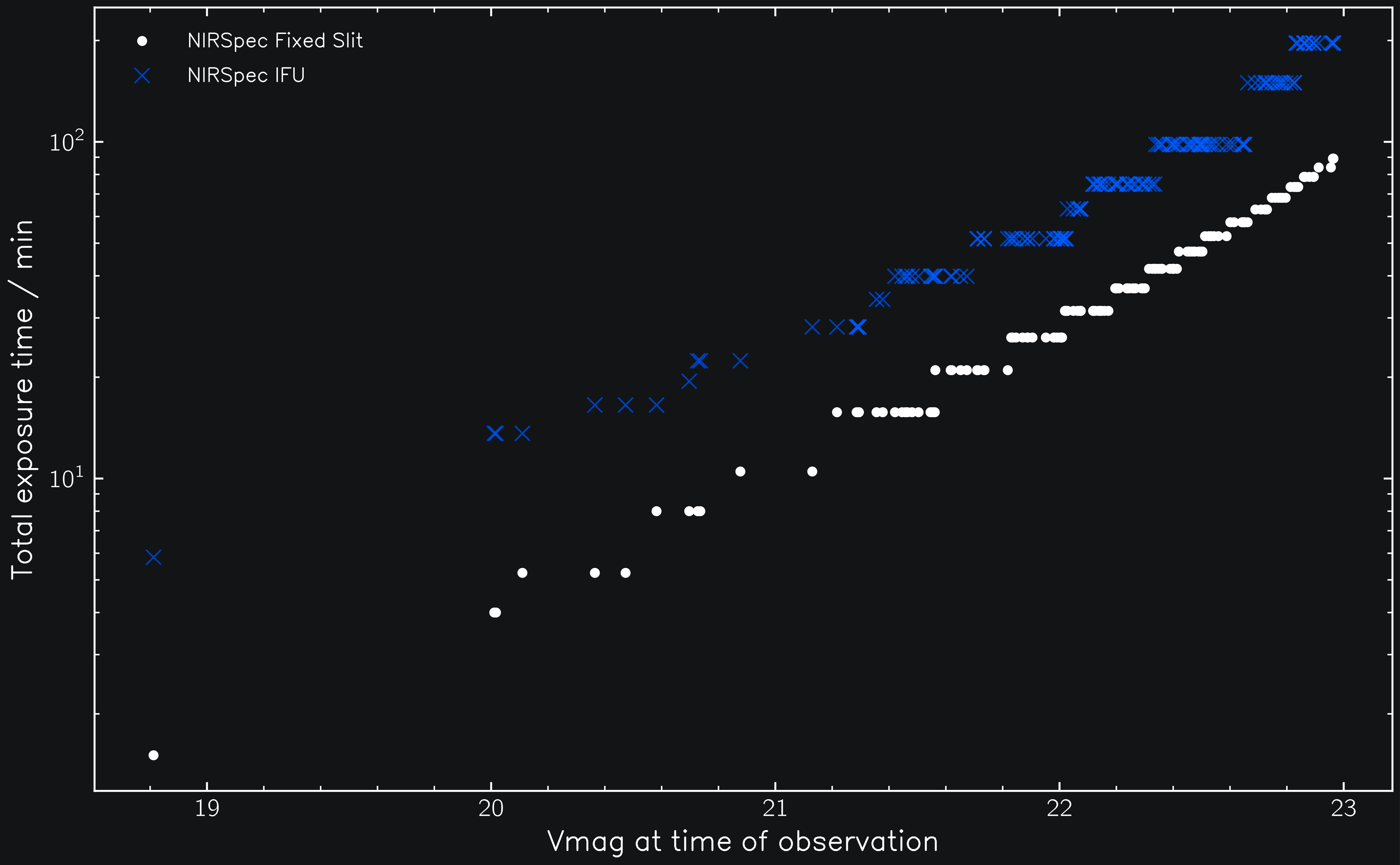
Fig. 5: Total exposure time to reach SNR=40-50 at 3μm versus apparent V magnitude for 149 classical TNOs during JWST Cycle 6.

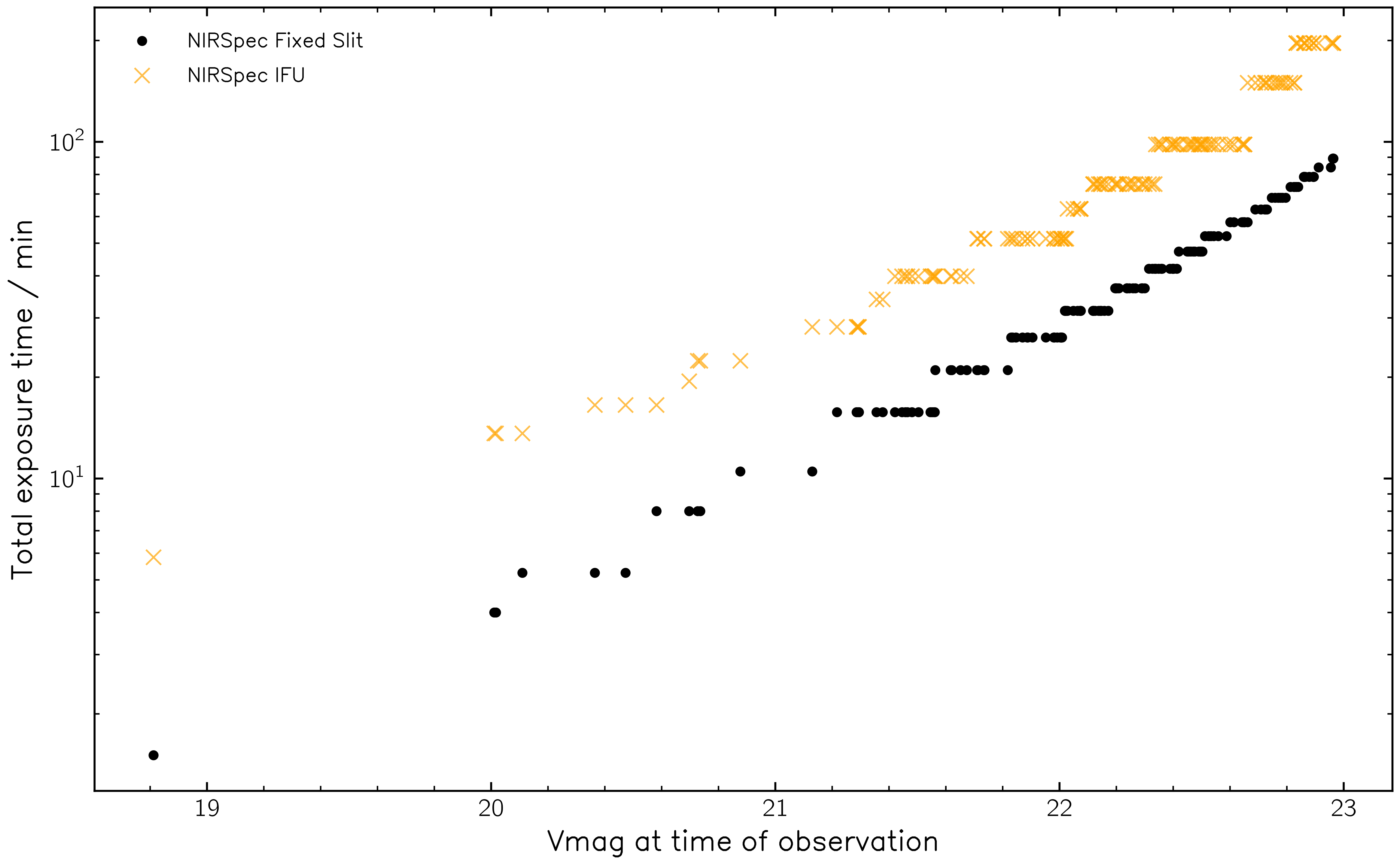
Fig. 5: Total exposure time to reach SNR=40-50 at 3μm versus apparent V magnitude for 149 classical TNOs during JWST Cycle 6.

On average, the IFU requires 2.2 times longer exposure times than Fixed Slit to reach the same SNR. The step-pattern in the exposure times is due to the discrete nature of the ngroup and nint settings.

---

At this point, we have all required information to plan our observations of classical TNOs with NIRSpec. The choice of IFU vs Fixed Slit mode for a given target will depend on its positional uncertainty, its brightness, and the available observing time.

---

[1]

Acronym underlining the importance of coffee when after long nights of disco and/or planning observations.