MIRI Observations of Vesta Family#
This tutorial outlines the observation planning for Vesta family members using the MIRI instrument during JWST Cycle 6. Our main objective is to study silicate composition, which requires achieving a target Signal-to-Noise Ratio (SNR) of 300 around 10μm. As the 10μm feature is accessible with both MIRI Low Resolution Spectrometer (LRS) and Medium Resolution Spectrometer (MRS), we use both modes.
We place the following constraints:
· Targets must be Vesta family members with a known diameter.
· The sample must span a range of diameters to encompass different sizes.
· Required SNR is 300 around 10μm.
Identifying potential targets#
We start by identifying all Vesta family members that have a known diameter, a
prerequisite for accurately modelling their thermal emission. We use the rocks
package to access the SsODNet/BFT asteroid database.
import rocks

# Load table of asteroid properties (SsODNet/BFT)
bft = rocks.load_bft()

# Select candidate targets: Vesta family members with known diameter
is_vestoid = bft["family.family_name"] == "Vesta"
has_diameter = bft["diameter.value"].notnull()

vestoids = bft[is_vestoid & has_diameter]
This initial selection yields 2041 Vesta family members with known diameters at the time of writing, all of which are potential targets.
Defining MIRI configurations#
We configure the MIRI MRS and LRS modes using jayrock, setting the optics,
exposure times, and readout patterns for each.
MRS Mode#
For the MRS, we set a standard 4-point dither (nexp=4). To target the 10μm
silicate feature, we initially set the aperture to Channel 2 and the Long
disperser.
import jayrock

miri_mrs = jayrock.Instrument('MIRI', mode='MRS')

miri_mrs.detector.nexp = 4  # 4-pt dither
miri_mrs.detector.readout_pattern = 'fastr1'  # recommended for MRS

miri_mrs.aperture = "ch2"
miri_mrs.disperser = "long"
LRS Mode#
We configure the LRS for SLIT mode and specify a 2-point dither (nexp=2). Since
LRS has only one valid optical component, no further configuration is required.
miri_lrs = jayrock.Instrument('MIRI', mode='LRSSLIT')

miri_lrs.detector.nexp = 2  # 2-pt dither
miri_lrs.detector.readout_pattern = 'fastr1'  # recommended for LRS
Determining observable diameters#
To understand the diameter range achievable with each MIRI mode, we select the largest Vesta family member within a set of representative diameter bins.
import pandas as pd

# ------
# Get largest Vestoid within diameter range
diameter_bins = [1, 2, 4, 8, 12, 16, 24, 32, 48, 64, 96, 128, 256, 512, 1024]

vestoids["diameter_bin"] = pd.cut(
    vestoids["diameter.value"], bins=diameter_bins, right=True, include_lowest=True
)

vestoids_largest_per_diameter_bin = vestoids.loc[
    vestoids.groupby("diameter_bin", observed=True)["diameter.value"].idxmax()
]
print(vestoids_largest_per_diameter_bin[["sso_name", "diameter.value", "diameter_bin"]])
   sso_name  diameter.value     diameter_bin
   2000 WE8           1.998     (0.999, 2.0]
 2000 QA163           3.995       (2.0, 4.0]
     Kollaa           7.922       (4.0, 8.0]
Koskenniemi          11.172      (8.0, 12.0]
       Mila          13.243     (12.0, 16.0]
 Robelmonte          23.834     (16.0, 24.0]
    Ausonia          93.000     (64.0, 96.0]
      Vesta         525.400  (512.0, 1024.0]
(4) Vesta is by far the largest family member, followed by (63) Ausonia at 93km diameter. No family members have sizes between 24 and 64km.
Estimating exposure times#
We now iterate through this sample to estimate the minimum exposure time
required to achieve an SNR between 300 and 400 at 10μm. Using an SNR range
(instead of a single value) speeds up the binary search, as the process stops
once any ngroup and nint combination is found. The resulting exposure
times are thus appropriate upper limits. Once we have our target list, we
will refine the exposure times further.
For each target, we:
Compute its ephemeris for Cycle 6.
Identify the date of minimum thermal flux (
thermal_min) during its visibility window, representing the most challenging observation scenario.Estimate the necessary exposure settings (
ngroupandnint) for both MRS and LRS modes.
# ------
# Estimate texp to reach SNR 300-400
for idx, asteroid in vestoids_largest_per_diameter_bin.iterrows():
    # Define target and compute ephemeris for JWST Cycle 6
    target = jayrock.Target(asteroid["sso_name"])
    target.compute_ephemeris(cycle=6)
    target.print_ephemeris()

    # Add total length of visibility windows to dataframe
    vestoids.loc[idx, "N_days_observable"] = len(target.ephemeris)

    # Get date of minimum thermal flux during visibility window
    date_obs = target.get_date_obs(at="thermal_min")

    # Compute exposure times for SNR targets
    for inst in [miri_mrs, miri_lrs]:
        # Estimate ngroup and nint
        success = inst.set_snr_target([300, 400], target, date_obs)

        if not success:
            print(f" Could not estimate SNR, skipping...")
            continue

        # Record results
        vestoids.loc[idx, f"nint_{inst.mode}"] = inst.detector.nint
        vestoids.loc[idx, f"ngroup_{inst.mode}"] = inst.detector.ngroup
        vestoids.loc[idx, f"texp_{inst.mode}"] = inst.texp
        vestoids.loc[idx, f"snr_{inst.mode}"] = inst.estimated_snr
Example outputs of these calculations for three targets are shown below.
The case of (2000) QA163
(2000) QA163 is observable with both MIRI MRS and LRS.
     (92804) 2000 QA163: Ephemeris from 2027-07-01 to 2028-06-30
     ├── Window 1: 2028-01-19 -> 2028-03-13
     │   ├── Duration         55 days
     │   ├── Vmag             21.03 -> 20.15
     │   └── Thermal @ 15um   14.05 -> 26.62 mJy
     ├── Window 2: 2028-05-29 -> 2028-06-30
     │   ├── Duration         33 days
     │   ├── Vmag             20.22 -> 20.81
     │   └── Thermal @ 15um   25.43 -> 17.07 mJy
     └── errRA/errDec in arcsec: 0.006 / 0.002
     # MIRI MRS SNR estimation
     INFO     [jayrock] Searching for minimum ngroup|nint to reach SNR range 300.0-400.0 at 10.85μm
     INFO     [jayrock]   nint=1 | ngroup=5   -> SNR=3.3   | Texp=0.9min
     INFO     [jayrock]   nint=1 | ngroup=100 -> SNR=176.2 | Texp=18.5min
     INFO     [jayrock]   nint=2 | ngroup=100 -> SNR=247.7 | Texp=37.2min
     INFO     [jayrock]   nint=3 | ngroup=100 -> SNR=301.5 | Texp=55.9min
     INFO     [jayrock] Done. Setting ngroup=100, nint=3.
     # MIRI LRS SNR estimation
     INFO     [jayrock] Searching for minimum ngroup|nint to reach SNR range 300.0-400.0 at 10.70μm
     INFO     [jayrock]   nint=1 | ngroup=5   -> SNR=25.7  | Texp=0.5min
     INFO     [jayrock]   nint=1 | ngroup=100 -> SNR=426.4 | Texp=9.3min
     INFO     [jayrock]   nint=1 | ngroup=52  -> SNR=308.1 | Texp=4.8min
     INFO     [jayrock] Done. Setting ngroup=52, nint=1.
The case of (63) Ausonia
(63) Ausonia is observable with MIRI MRS but saturates in LRS mode.
# Ephemeris query results
(63) Ausonia: Ephemeris from 2027-07-01 to 2028-06-30
├── Window 1: 2027-12-22 -> 2028-02-16
│   ├── Duration         57 days
│   ├── Vmag             11.93 -> 10.84
│   └── Thermal @ 15um   7667.04 -> 18441.00 mJy
├── Window 2: 2028-05-02 -> 2028-06-30
│   ├── Duration         60 days
│   ├── Vmag             10.61 -> 11.48
│   └── Thermal @ 15um   23630.42 -> 12551.21 mJy
└── errRA/errDec in arcsec: 0.011 / 0.007

# MIRI MRS SNR estimation
INFO     [jayrock] Searching for minimum ngroup|nint to reach SNR range 300.0-400.0 at 10.85μm
INFO     [jayrock]   nint=1 | ngroup=5   -> SNR=596.3 | Texp=0.9min
INFO     [jayrock] Done. Setting ngroup=5, nint=1.
# MIRI LRS SNR estimation
INFO     [jayrock] Searching for minimum ngroup|nint to reach SNR range 300.0-400.0 at 10.70μm
WARNING  [jayrock] Observation warnings: {'full_saturated': 'Full saturation:\n There are 879 pixels saturated at
         the end of the first group. These pixels cannot be recovered.', 'partial_saturated': 'Partial
         saturation:\n There are 335 pixels saturated at the end of a ramp. Partial ramps may still be used in some
         cases.'}
WARNING  [jayrock]   nint=1 | ngroup=5   -> FULL SATURATION.
ERROR    [jayrock] Minimum nint/ngroup saturated. Stopping search. Providing parameter 'bounds' might avoid this.
 Could not estimate SNR, skipping...
The case of (4) Vesta
(4) Vesta saturates even with the lowest possible ngroup and nint settings in both MIRI MRS and LRS.
# Ephemeris query results
(4) Vesta: Ephemeris from 2027-07-01 to 2028-06-30
├── Window 1: 2027-11-01 -> 2027-12-26
│   ├── Duration         56 days
│   ├── Vmag             8.05 -> 7.08
│   └── Thermal @ 15um   215806.57 -> 464579.59 mJy
├── Window 2: 2028-03-10 -> 2028-05-06
│   ├── Duration         58 days
│   ├── Vmag             6.99 -> 7.83
│   └── Thermal @ 15um   519366.32 -> 273551.43 mJy
└── errRA/errDec in arcsec: 0.017 / 0.001

# MIRI MRS SNR estimation
INFO     [jayrock] Searching for minimum ngroup|nint to reach SNR range 300.0-400.0 at 10.85μm
WARNING  [jayrock] Observation warnings: {'ifu_full_saturated': 'Full saturation:\n In the current wavelength
         slice, there are 1 pixels saturated at the end of the first group. These pixels cannot be recovered.',
         'ifu_partial_saturated': 'Partial saturation:\n In the current wavelength slice, there are 4 pixels
         saturated at the end of a ramp. Partial ramps may still be used in some cases.', 'cube_full': 'There are
         6730 total fully saturated pixels in the data cube.', 'cube_partial': 'There are 1839 total partially
         saturated pixels in the data cube.'}
WARNING  [jayrock]   nint=1 | ngroup=5   -> FULL SATURATION.
ERROR    [jayrock] Minimum nint/ngroup saturated. Stopping search. Providing parameter 'bounds' might avoid this.
 Could not estimate SNR, skipping...
# MIRI LRS SNR estimation
INFO     [jayrock] Searching for minimum ngroup|nint to reach SNR range 300.0-400.0 at 10.70μm
WARNING  [jayrock] Observation warnings: {'full_saturated': 'Full saturation:\n There are 3602 pixels saturated at
         the end of the first group. These pixels cannot be recovered.', 'partial_saturated': 'Partial
         saturation:\n There are 1389 pixels saturated at the end of a ramp. Partial ramps may still be used in
         some cases.'}
WARNING  [jayrock]   nint=1 | ngroup=5   -> FULL SATURATION.
ERROR    [jayrock] Minimum nint/ngroup saturated. Stopping search. Providing parameter 'bounds' might avoid this.
The table below shows the exposure times (in seconds). A value of NaN indicates
that the target saturates even at the minimum exposure settings.
   sso_name  diameter.value     texp_mrs  texp_lrsslit
   2000 WE8           1.998  15684.52608    1115.56608
 2000 QA163           3.995   3352.24832     288.60416
     Kollaa           7.922   1110.01600      88.80128
Koskenniemi          11.172    577.20832      55.50080
       Mila          13.243    577.20832      55.50080
 Robelmonte          23.834     77.70112           NaN
    Ausonia          93.000     55.50080           NaN
      Vesta         525.400          NaN           NaN
The exposure times confirm that MIRI MRS (IFU mode) is less sensitive than MIRI LRS (slit mode). MRS can observe larger, brighter targets without saturation, yet it requires considerably longer exposure times for the smaller targets compared to LRS. LRS saturates for targets larger than ∼24 km, and Vesta saturates in both modes.
We can visualise this trade-off by plotting the exposure time against the diameter:
import matplotlib.pyplot as plt

fig, ax = plt.subplots()

ax.scatter(
    vestoids_largest_per_diameter_bin["diameter.value"],
    vestoids_largest_per_diameter_bin["texp_mrs"] / 60,
    label="MIRI MRS",
    s=50,
)

ax.scatter(
    vestoids_largest_per_diameter_bin["diameter.value"],
    vestoids_largest_per_diameter_bin["texp_lrsslit"] / 60,
    label="MIRI LRS",
    s=50,
    marker="s"
)

ax.set(xscale="log", yscale="log", xlabel="Diameter / km", ylabel="Exposure time / min")
ax.legend()
plt.show()
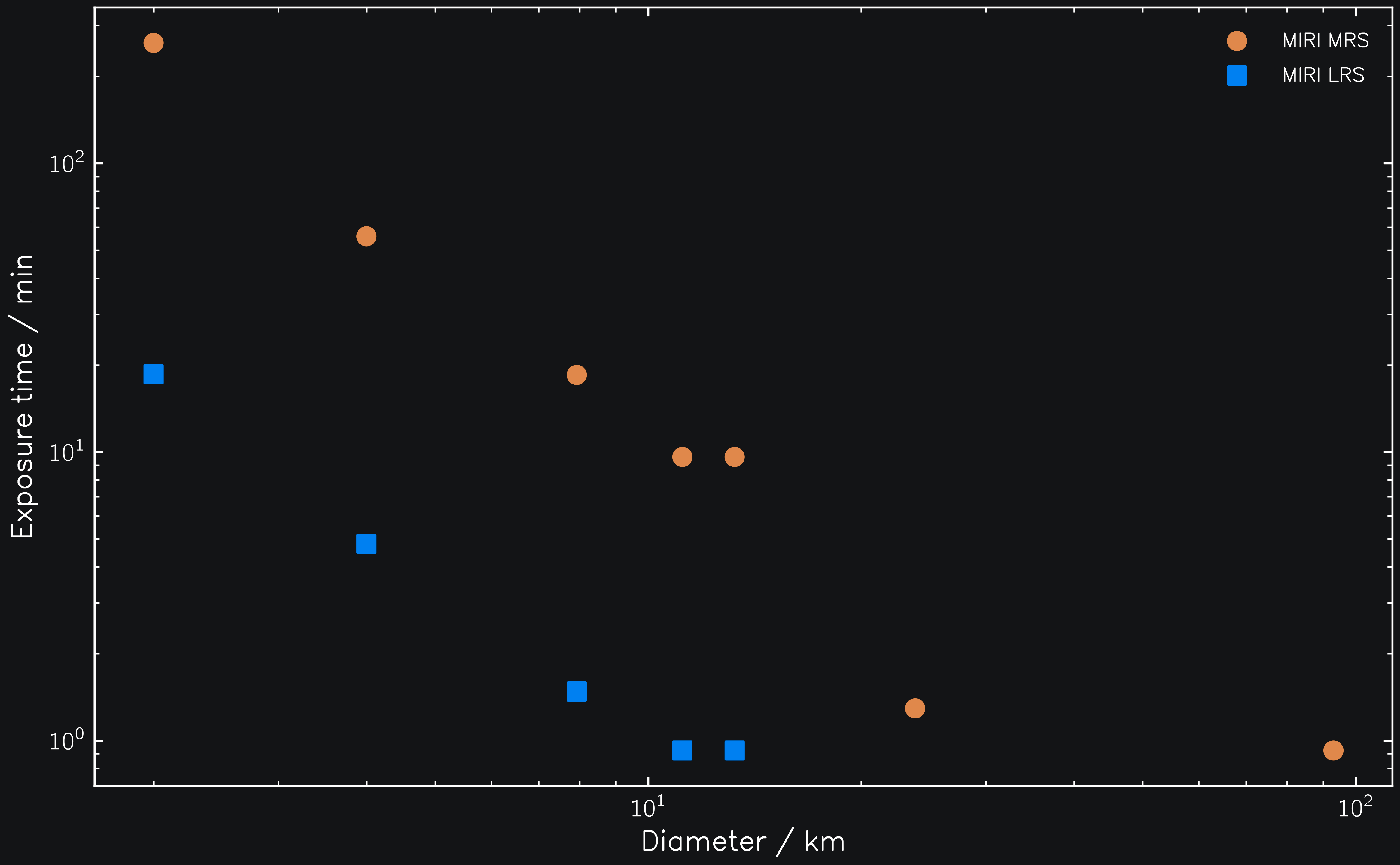
Fig. 1: Required total exposure times for SNRs between 300-400 versus diameter for selected Vestoids.#
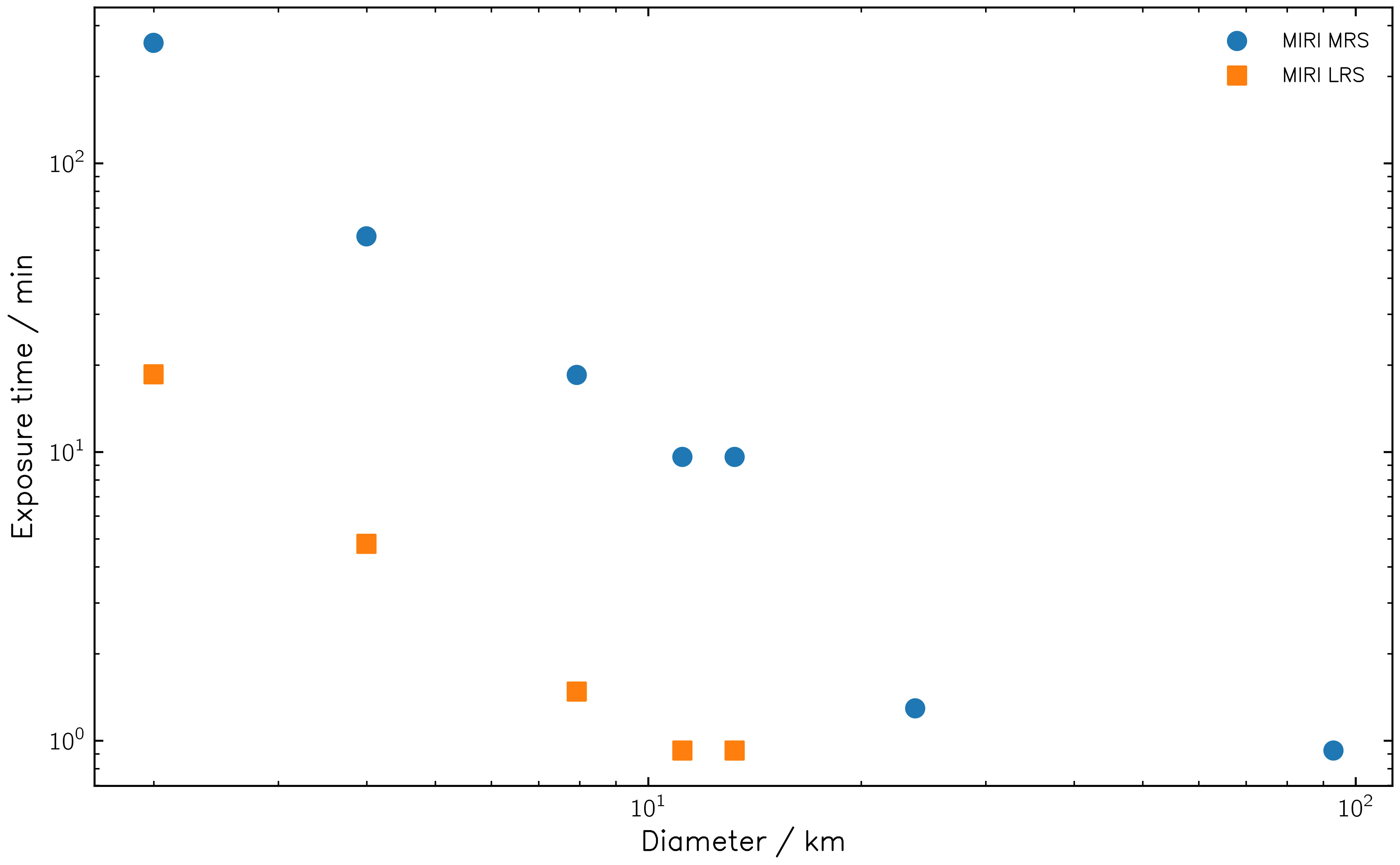
Fig. 1: Required total exposure times for SNRs between 300-400 versus diameter for selected Vestoids.#
Defining final observing strategy#
Based on the exposure time analysis:
· MIRI MRS is suitable for targets down to approximately 4km diameter to meet the SNR requirement within a reasonable exposure time.
· MIRI LRS is necessary for the smallest targets, those <4km.
For this example, we select the five targets ranging from 8km to 93km for observations in MRS mode and the two targets under 4km for observations in LRS mode.
Configuring MRS mode#
For MRS, we must calculate the required exposure settings across all four
channels and three dispersers. Channels 2 and 3 cover the key silicate
features, so we set their target SNR to 300. Channel 4 is less sensitive and is
set to SNR 100. For Channel 1, which has low throughput and is observed
concurrently with Channel 2, we use the minimum exposure settings (ngroup=5,
nint=1).
TARGETS_MRS = ["Kollaa", "Koskenniemi", "Mila", "Robelmonte", "Ausonia"]

SNR_targets = {
    'ch2': {'short': 300, 'medium': 300, 'long': 300},
    'ch3': {'short': 300, 'medium': 300, 'long': 300},
    'ch4': {'short': 100, 'medium': 100, 'long': 100},
}
We now loop over our targets and instrument configurations to compute the
required nint and ngroup for the APT. We always use 4-point dithers
(nexp=4) for the target observations. We store these parameters in a
dictionary to avoid recomputing them later.
MRS_OBSERVING_PARAMETERS = {}

for target in TARGETS_MRS:
    # Define target and compute ephemeris for JWST Cycle 6
    target = jayrock.Target(target)
    target.compute_ephemeris(cycle=6)

    # Get date of minimum thermal flux during visibility window
    date_obs = target.get_date_obs(at="thermal_min")

    for channel in ["ch1", "ch2", "ch3", "ch4"]:
        for disperser in ["short", "medium", "long"]:
            # Set aperture and disperser
            miri_mrs.aperture = channel
            miri_mrs.disperser = disperser

            if channel == "ch1":
                # Use minimum ngroup/nint
                miri_mrs.detector.ngroup = 5
                miri_mrs.detector.nint = 1
            else:
                # Get SNR target
                snr_target = SNR_targets[channel][disperser]
                # Estimate ngroup and nint based on SNR target
                miri_mrs.set_snr_target(snr_target, target, date_obs)

            print(
                f"{target.name:15s} | {channel:3s} | {disperser:6s} | "
                f"ngroup: {miri_mrs.detector.ngroup:2d} | nint: {miri_mrs.detector.nint:2d} | "
                f"texp: {miri_mrs.texp / 60:6.2f} min"
            )

            if target.name not in MRS_OBSERVING_PARAMETERS:
                MRS_OBSERVING_PARAMETERS[target.name] = {}

            MRS_OBSERVING_PARAMETERS[target.name][(channel, disperser)] = {
                "ngroup": miri_mrs.detector.ngroup,
                "nint": miri_mrs.detector.nint,
            }
MRS_OBSERVING_PARAMETERS = {
 "Kollaa": {
     ("ch1", "short"): {"ngroup": 5, "nint": 1},
     ("ch1", "medium"): {"ngroup": 5, "nint": 1},
     ("ch1", "long"): {"ngroup": 5, "nint": 1},
     ("ch2", "short"): {"ngroup": 83, "nint": 4},
     ("ch2", "medium"): {"ngroup": 69, "nint": 2},
     ("ch2", "long"): {"ngroup": 74, "nint": 1},
     ("ch3", "short"): {"ngroup": 62, "nint": 1},
     ("ch3", "medium"): {"ngroup": 47, "nint": 1},
     ("ch3", "long"): {"ngroup": 40, "nint": 1},
     ("ch4", "short"): {"ngroup": 28, "nint": 1},
     ("ch4", "medium"): {"ngroup": 48, "nint": 1},
     ("ch4", "long"): {"ngroup": 91, "nint": 3},
 },
 "Koskenniemi": {
     ("ch1", "short"): {"ngroup": 5, "nint": 1},
     ("ch1", "medium"): {"ngroup": 5, "nint": 1},
     ("ch1", "long"): {"ngroup": 5, "nint": 1},
     ("ch2", "short"): {"ngroup": 86, "nint": 2},
     ("ch2", "medium"): {"ngroup": 72, "nint": 1},
    # ...
    },
    # ...
}
Checking SNR and saturation#
We check the full SNR curve at both the date of minimum and maximum thermal flux to confirm the observation avoids saturation across the full visibility window.
for target, params in MRS_OBSERVING_PARAMETERS.items():
    observations = []

    print(f"Target: {target}")
    target = jayrock.Target(target)
    target.compute_ephemeris(cycle=6)

    date_obs_thermal_min = target.get_date_obs(at="thermal_min")
    date_obs_thermal_max = target.get_date_obs(at="thermal_max")

    for (channel, disperser), settings in params.items():
        ngroup = settings["ngroup"]
        nint = settings["nint"]

        miri_mrs.aperture = channel
        miri_mrs.disperser = disperser
        miri_mrs.detector.ngroup = ngroup
        miri_mrs.detector.nint = nint

        obs_thermal_min = jayrock.observe(target, miri_mrs, date_obs_thermal_min)
        obs_thermal_max = jayrock.observe(target, miri_mrs, date_obs_thermal_max)
        observations.append(obs_thermal_min)
        observations.append(obs_thermal_max)

    # Save plot to file
    jayrock.plot_snr(
        observations, show=False, save_to=f"{target.name}_miri_mrs_snr.ng"
    )
SNR of (1929) Kollaa
Below is the SNR plot for (1929) Kollaa at both the minimum and maximum thermal flux dates. All SNR targets are reached without saturation at both dates. Channel 1 will not yield much information, however, it is observed “for free” with channel 2.
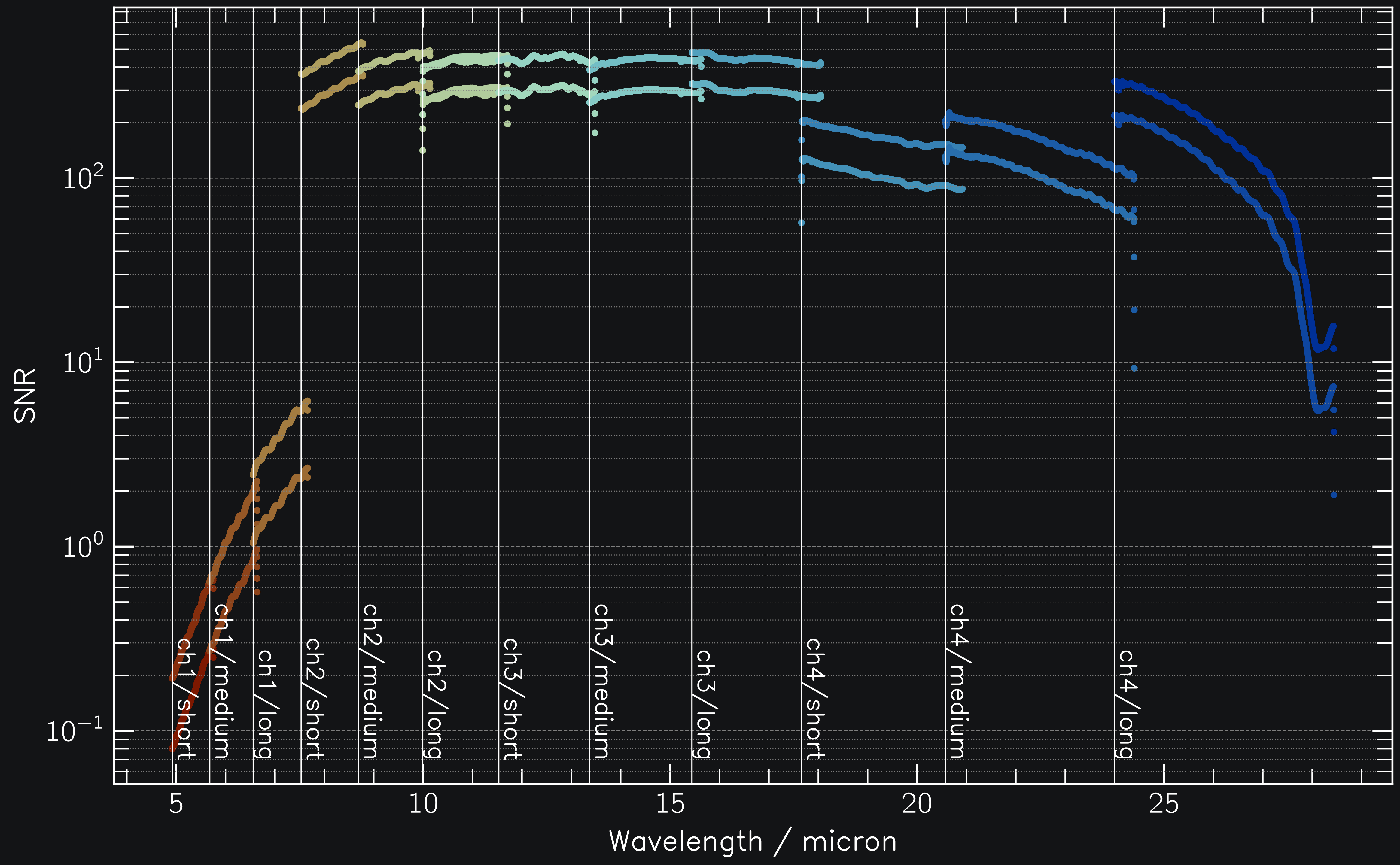
Fig. 2: SNR of MIRI observations of (1929) Kollaa.#
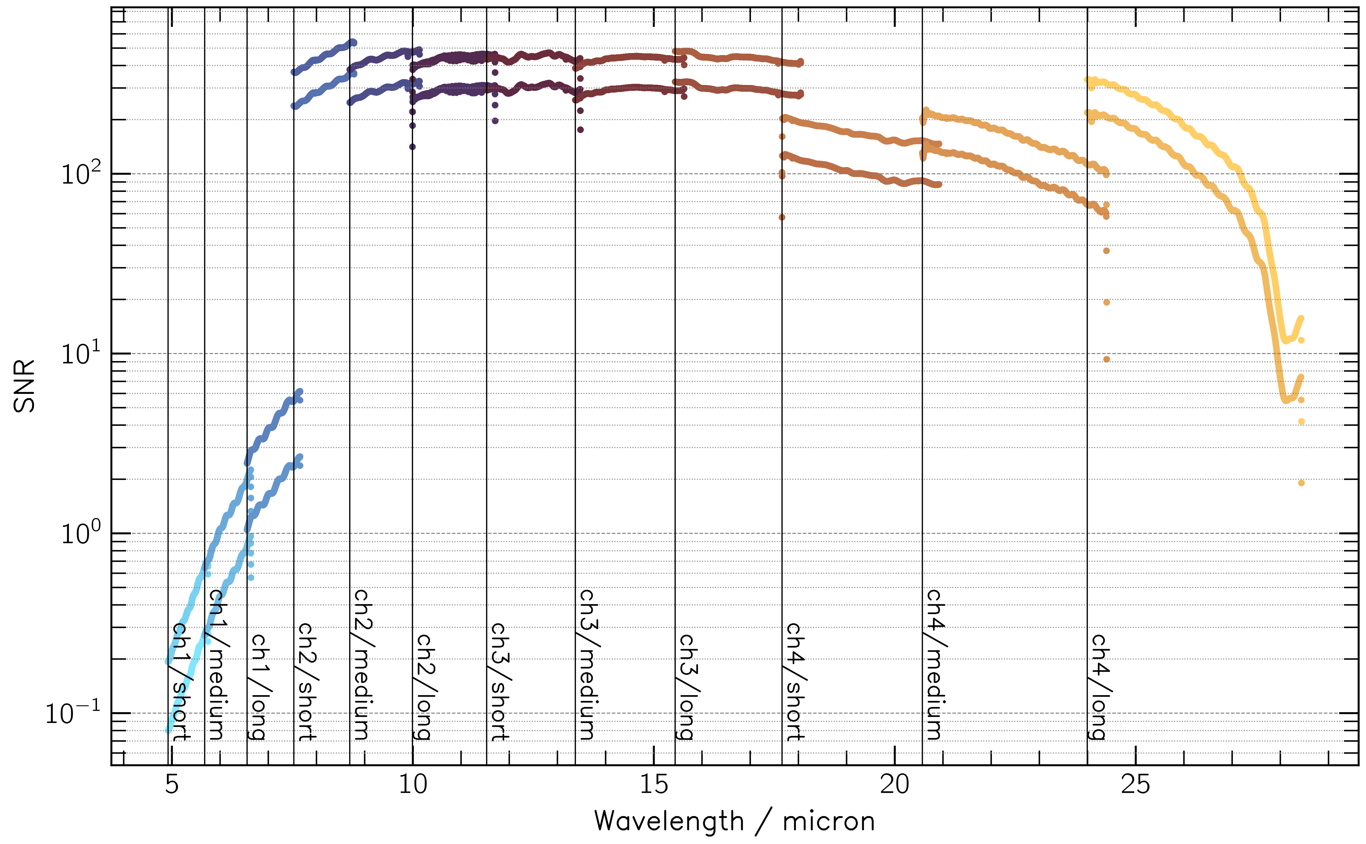
Fig. 2: SNR of MIRI observations of (1929) Kollaa.#
SNR of (63) Ausonia
(63) Ausonia is saturating in channels 2 and 3 at the dates of maximum thermal flux.
This is shown in the console log (not shown here) and in the figure below, where only one
SNR curve is plotted in these channels (SNR is NaN in case of saturation).
We already use the minimum recommended ngroup, nint, and nexp values for
this target. In this case, we could either go below (eg go towards a
2-point dither pattern) or restrict the observations to dates of low
thermal flux only. This is left as exercise to the reader.
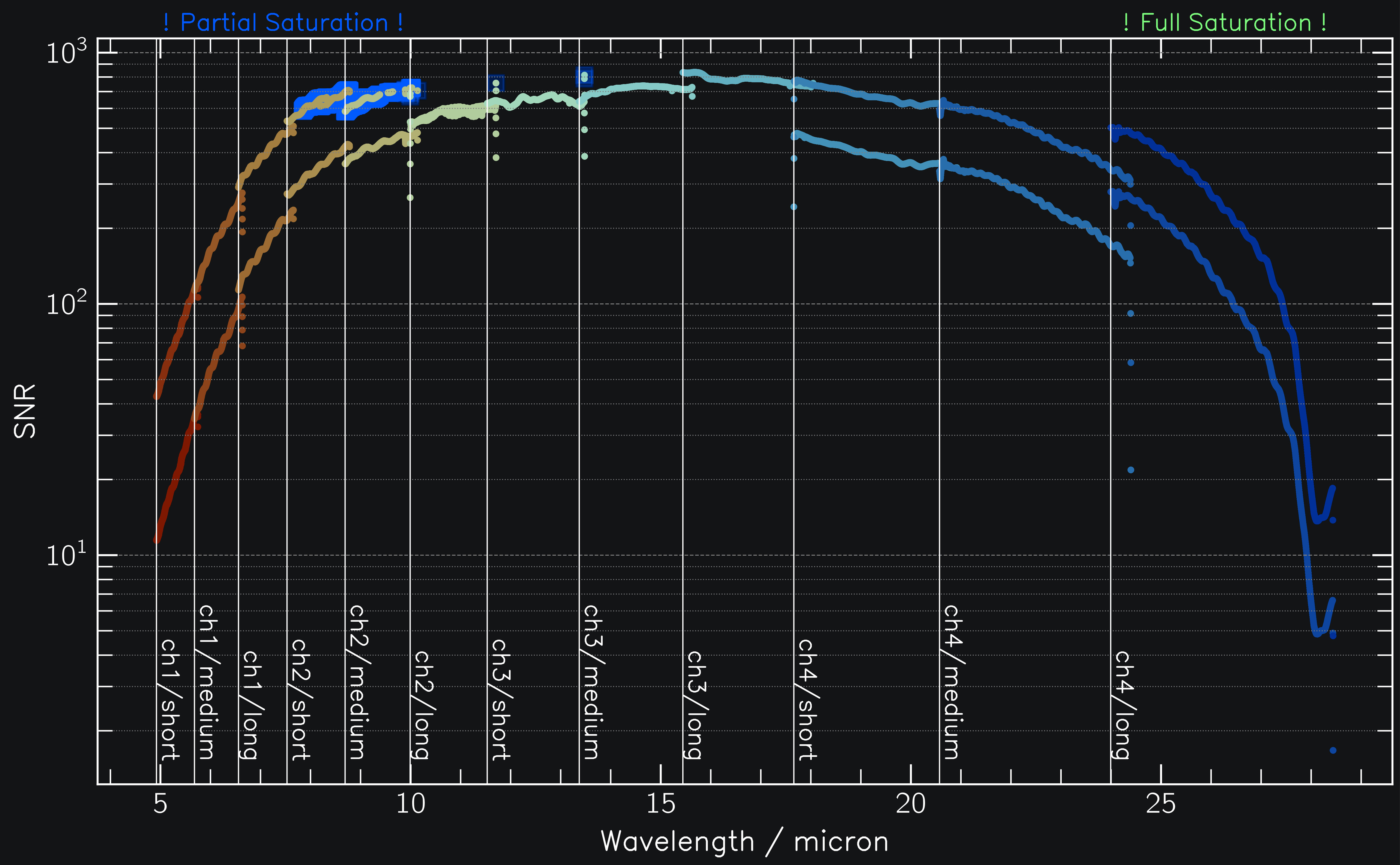
Fig. 3: SNR of MIRI observations of (63) Ausonia.#
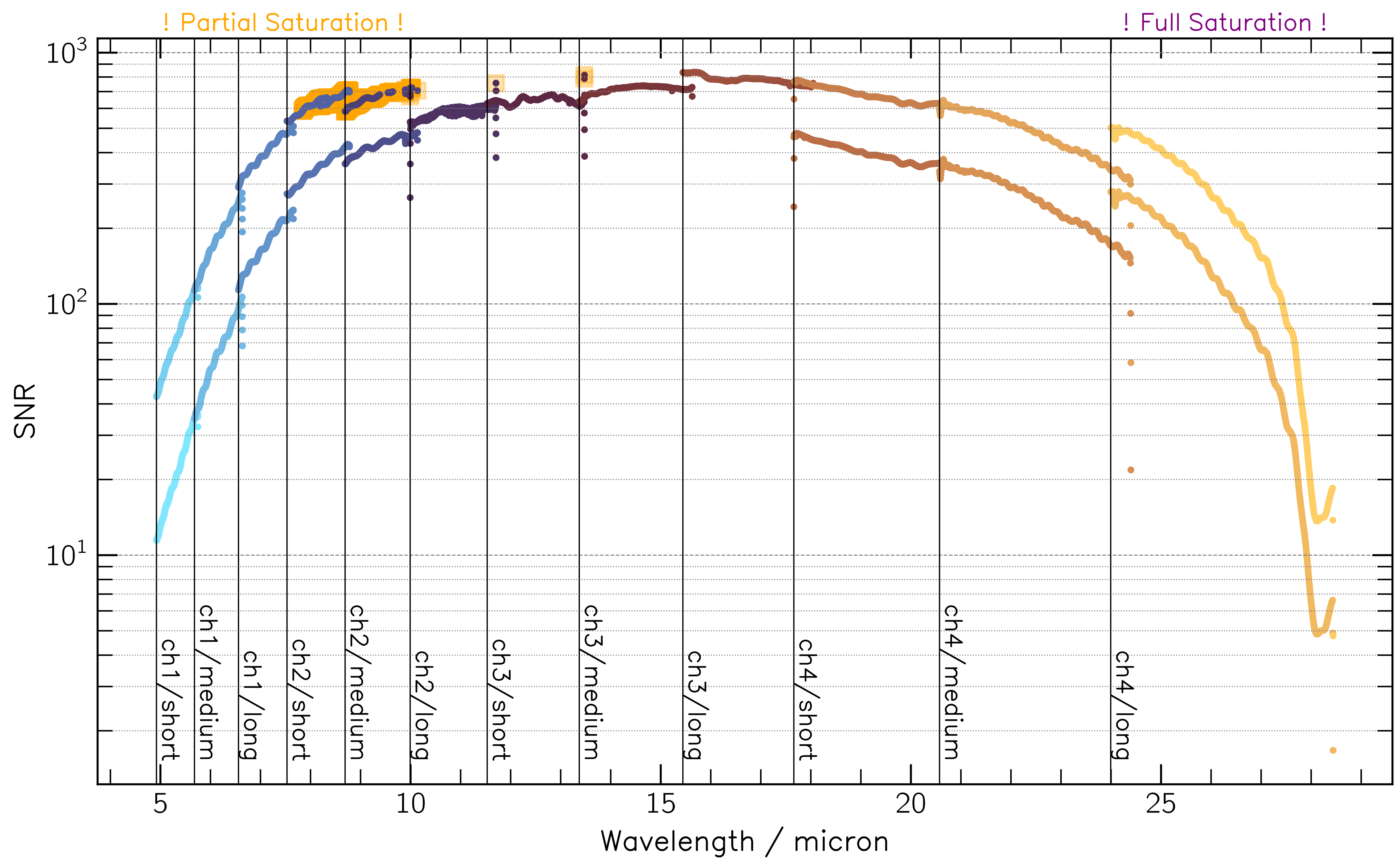
Fig. 3: SNR of MIRI observations of (63) Ausonia.#
Configuring LRS mode#
We calculate the settings for the two smallest targets using MIRI LRS, aiming for an SNR of 300 at 10μm.
TARGETS_LRS = ["2000 WE8", "2000 QA163"]
SNR_TARGET = 300

LRS_OBSERVING_PARAMETERS = {}

for target in TARGETS_LRS:
    # Define target and compute ephemeris for JWST Cycle 6
    target = jayrock.Target(target)
    target.compute_ephemeris(cycle=6)

    # Get date of minimum thermal flux during visibility window
    date_obs = target.get_date_obs(at="thermal_min")

    # Compute exposure times for SNR target at 10 micron
    miri_lrs.set_snr_target(SNR_TARGET, target, date_obs, wave=10)

    print(
        f"{target.name:15s} | "
        f"ngroup: {miri_lrs.detector.ngroup:2d} | nint: {miri_lrs.detector.nint:2d} | "
        f"texp: {miri_lrs.texp / 60:6.2f} min"
    )

    LRS_OBSERVING_PARAMETERS[target.name] = {
        "ngroup": miri_lrs.detector.ngroup,
        "nint": miri_lrs.detector.nint,
    }
LRS_OBSERVING_PARAMETERS = {
    "2000 WE8": {"ngroup": 65, "nint": 2},
    "2000 QA163": {"ngroup": 36, "nint": 1},
}
Checking SNR and saturation#
We confirm that the LRS observations also avoid saturation at the date of highest thermal emission.
for target, params in LRS_OBSERVING_PARAMETERS.items():
    observations = []

    print(f"Target: {target}")
    target = jayrock.Target(target)
    target.compute_ephemeris(cycle=6)

    date_obs_thermal_min = target.get_date_obs(at="thermal_min")
    date_obs_thermal_max = target.get_date_obs(at="thermal_max")

    miri_lrs.detector.ngroup = params["ngroup"]
    miri_lrs.detector.nint = params["nint"]

    obs_thermal_min = jayrock.observe(target, miri_lrs, date_obs_thermal_min)
    obs_thermal_max = jayrock.observe(target, miri_lrs, date_obs_thermal_max)
    observations.append(obs_thermal_min)
    observations.append(obs_thermal_max)

    # Save plot to file
    jayrock.plot_snr(
        observations, show=False, save_to=f"{target.name}_miri_lrs_snr.png"
    )
The results show no saturation issues for the two small LRS targets at either thermal extreme.
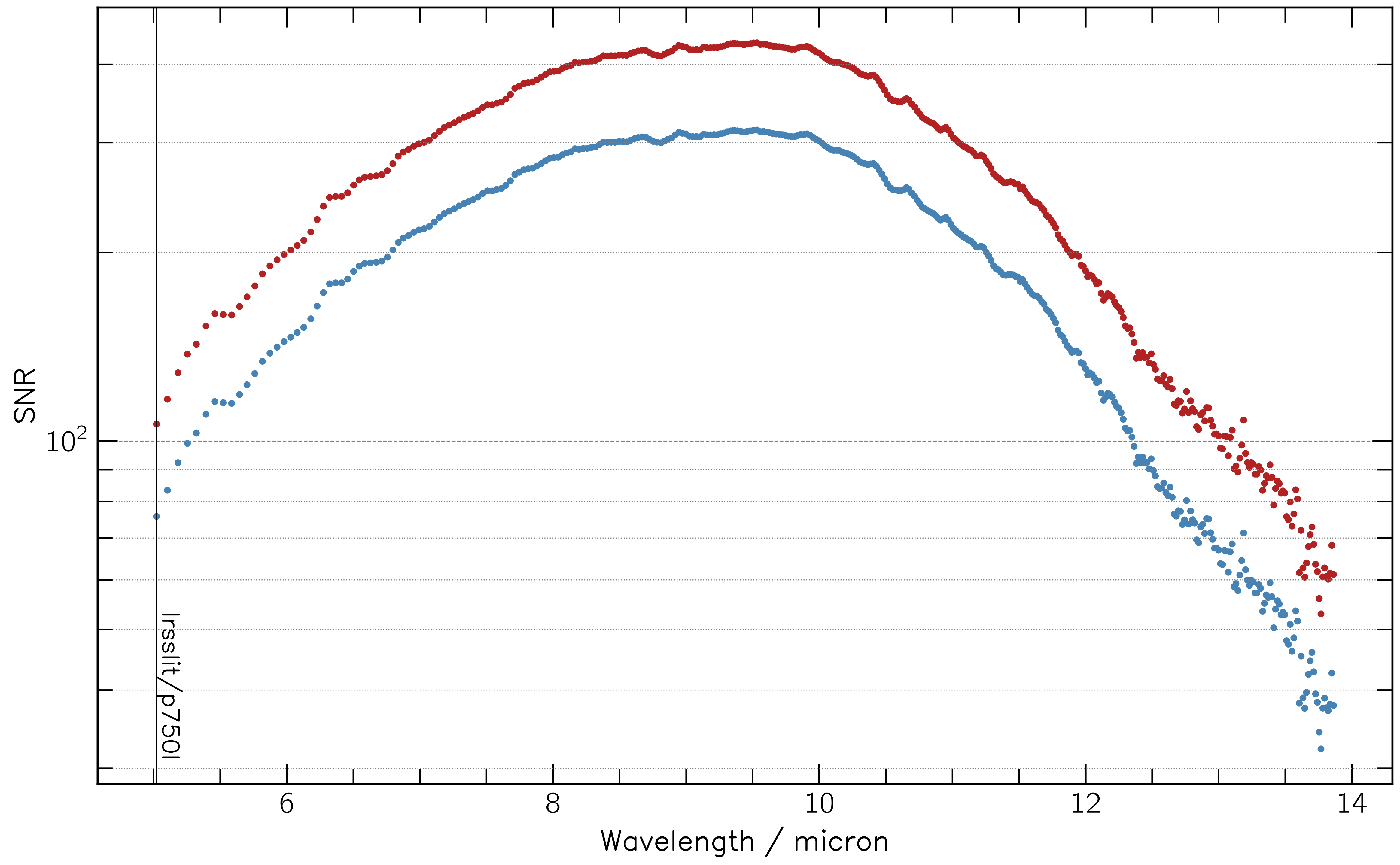
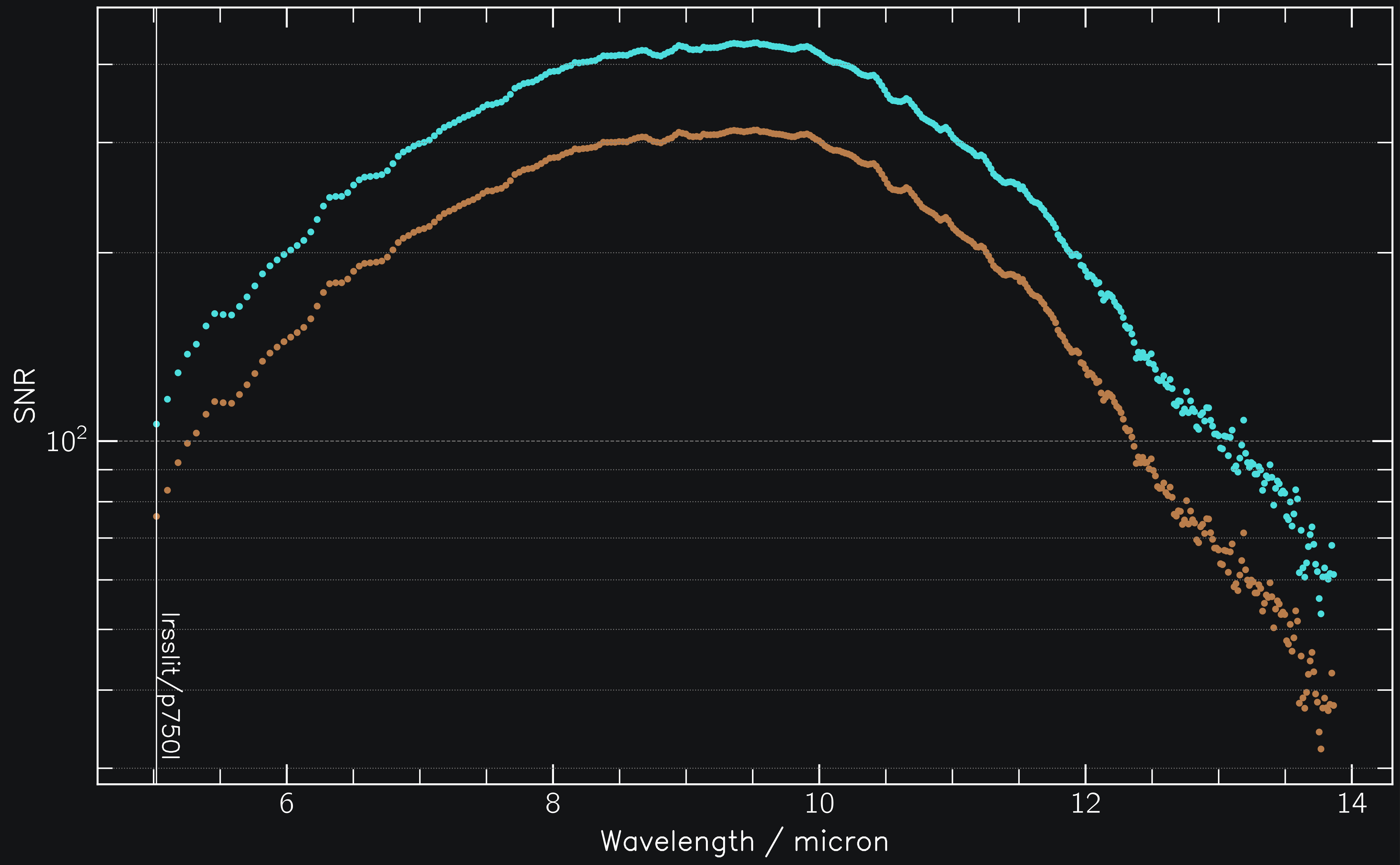
SNR of (2000) QA163
Verification with JWST ETC and APT#
The MRS_OBSERVING_PARAMETERS and LRS_OBSERVING_PARAMETERS dictionaries
contain all required information to set up the observations in APT. To verify
that the SNRs and saturation levels match between Jayrock and the JWST ETC, we
can export the spectra for each target and import them into the ETC.
TARGETS = TARGETS_MRS + TARGETS_LRS

for target in TARGETS:
    target = jayrock.Target(target)
    target.compute_ephemeris(cycle=6)

    date_obs = target.get_date_obs(at="thermal_min")
    target.export_spectrum(f"{target.name}_spectrum_thermal_minimum.txt", date_obs=date_obs)