Identify your Target

Identify your Target#

The jayrock.Target class handles identification, gathering physical properties, and calculating orbital visibility/fluxes (ephemeris) for your minor body as seen from JWST.

Defining a Target#

Identify your target by passing a name, designation, or number. jayrock uses rocks to automatically retrieve available physical parameters.

import jayrock
luisa = jayrock.Target('Luisa')        # (599) Luisa
chariklo = jayrock.Target('1997 CU26') # (10199) Chariklo
pluto = jayrock.Target(134340)         # (134340) Pluto

Get ephemeris as seen from JWST#

After defining the target, we want to know whether it is observable from JWST during a given timeframe (cycle) and at what visual magnitude / thermal flux we can observe it. The compute_ephemeris() method computes visibility windows and fluxes using jwst_gtvt and JPL Horizons.

# Ephemeris of (599) Luisa for Cycle 6 (2027-07-01 - 2028-06-30)
luisa.compute_ephemeris(cycle=6)

The result of the query is stored in the ephemeris attribute of the target, a pandas.DataFrame. Each row in the dataframe represents one date on which the target is visible and contains viewing geometry, fluxes, and more. To get a high-level overview, use the print_ephemeris() method:

>>> luisa.print_ephemeris()
(599) Luisa: Ephemeris from 2027-07-01 to 2028-06-30
├── Window 1: 2027-07-12 -> 2027-09-17
│   ├── Duration         68 days
│   ├── Vmag             12.72 -> 11.68
│   └── Thermal @ 15um   12657.03 -> 26584.46 mJy
├── Window 2: 2027-12-02 -> 2028-01-31
│   ├── Duration         61 days
│   ├── Vmag             12.18 -> 13.55
│   └── Thermal @ 15um   16169.68 -> 5146.10 mJy
└── errRA/errDec in arcsec: 0.015 / 0.013

Warning

Visibility windows can slightly vary between those obtained by the APT and those obtained here with jwst_mtvt (order of one day). The APT has the final authority.

The queries to JPL Horizons are executed with astroquery and use the built-in cache system. By default, the cache resets after 7 days.

Select a date of observation#

Simulating an observation requires a date of observation date_obs. You can retrieve all possible dates withe the get_date_obs() method or select one based on brightness criteria using the at argument.

>>> dates_obs = luisa.get_date_obs()  # gets all valid date_obs
>>> print(dates_obs)
['2027-07-12', '2027-07-13', '2027-07-14', ..., '2028-01-29', '2028-01-30', '2028-01-31']
>>> date_obs = luisa.get_date_obs(at="vmag_min")  # gets date_obs at minimum V magnitude
>>> print(date_obs)
'20207-09-17'

Valid conditions are vmag_min, vmag_max, thermal_min, thermal_max.

Modelling the spectrum#

Target spectra are modelled as superposition of a reflected and a thermal component.

Reflected Component#

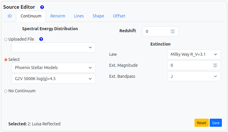
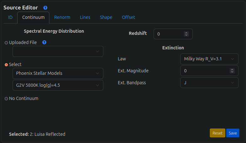
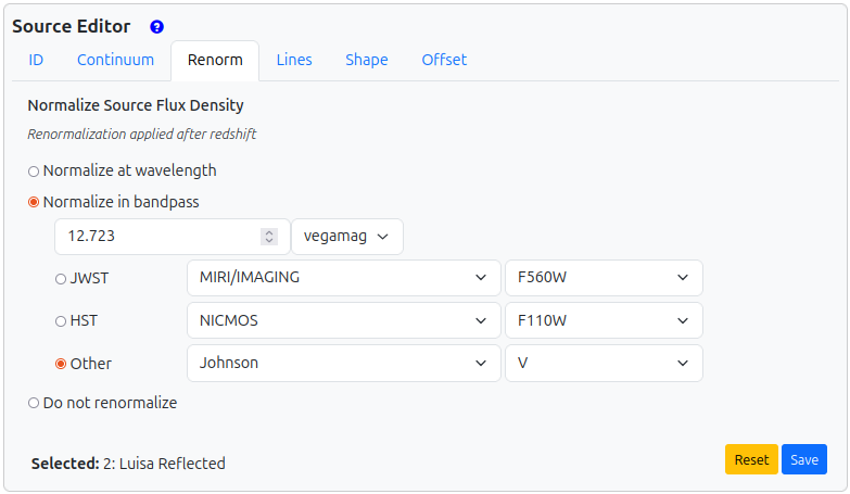
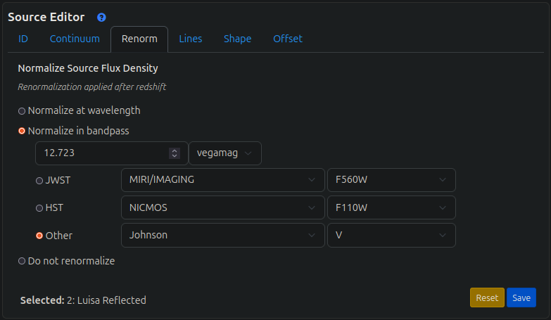
The reflected component of the minor planet is modeled using a Phoenix stellar model of a G2V star. The spectrum is normalised to the apparent Johnson V magnitude as seen from JWST on the date of observation. This setup can be replicated in the ETC in the following way:

Source Editor - Continuum

Source Editor - Renorm

Thermal Component#

The thermal component is modelled via the Near-Earth Asteroid Thermal Model (NEATM) by Harris (1998). The implementation in jayrock is essentially a copy of the code in Michael Kelley’s mskpy. The following parameters are required to model the target’s spectrum. If the parameter is unknown (i.e. not available via rocks), jayrock assumes the given default value.

Name	Description	Default
albedo	Target geometrical albedo in V.	0.1
diameter	Target diameter in km.	30
beaming (\(\eta\))	Parameter accounting for surface roughness and thermal inertia effects.	1.0
emissivity (\(\epsilon\))	Ratio of asteroid’s thermal radiation to ideal blackbody’s radiation.	0.9

You can override the default values using the dot-notation.

luisa.albedo = 0.11
luisa.diameter = 68
luisa.beaming = 1
luisa.emissivity = 1

Exporting and plotting#

Export the full spectrum or individual components (e.g. for verification with the online ETC):

luisa.export_spectrum('luisa_spectrum.txt', date_obs='2027-12-24')
luisa.export_spectrum('luisa_spectrum_refl.txt', date_obs='2027-12-24', thermal=False)  # only reflected component
luisa.export_spectrum('luisa_spectrum_thermal.txt', date_obs='2027-12-24', reflected=False)  # only thermal component

Plot the spectrum of a target at a given date_obs:

luisa.plot_spectrum(date_obs='2027-12-24')

You can provide a list of date_obs to compare the fluxes at different dates.

  date_vmag_min = luisa.get_date_obs(at='vmag_min')
  date_vmag_max = luisa.get_date_obs(at='vmag_max')
  luisa.plot_spectrum(date_obs=[date_vmag_min, date_vmag_max])

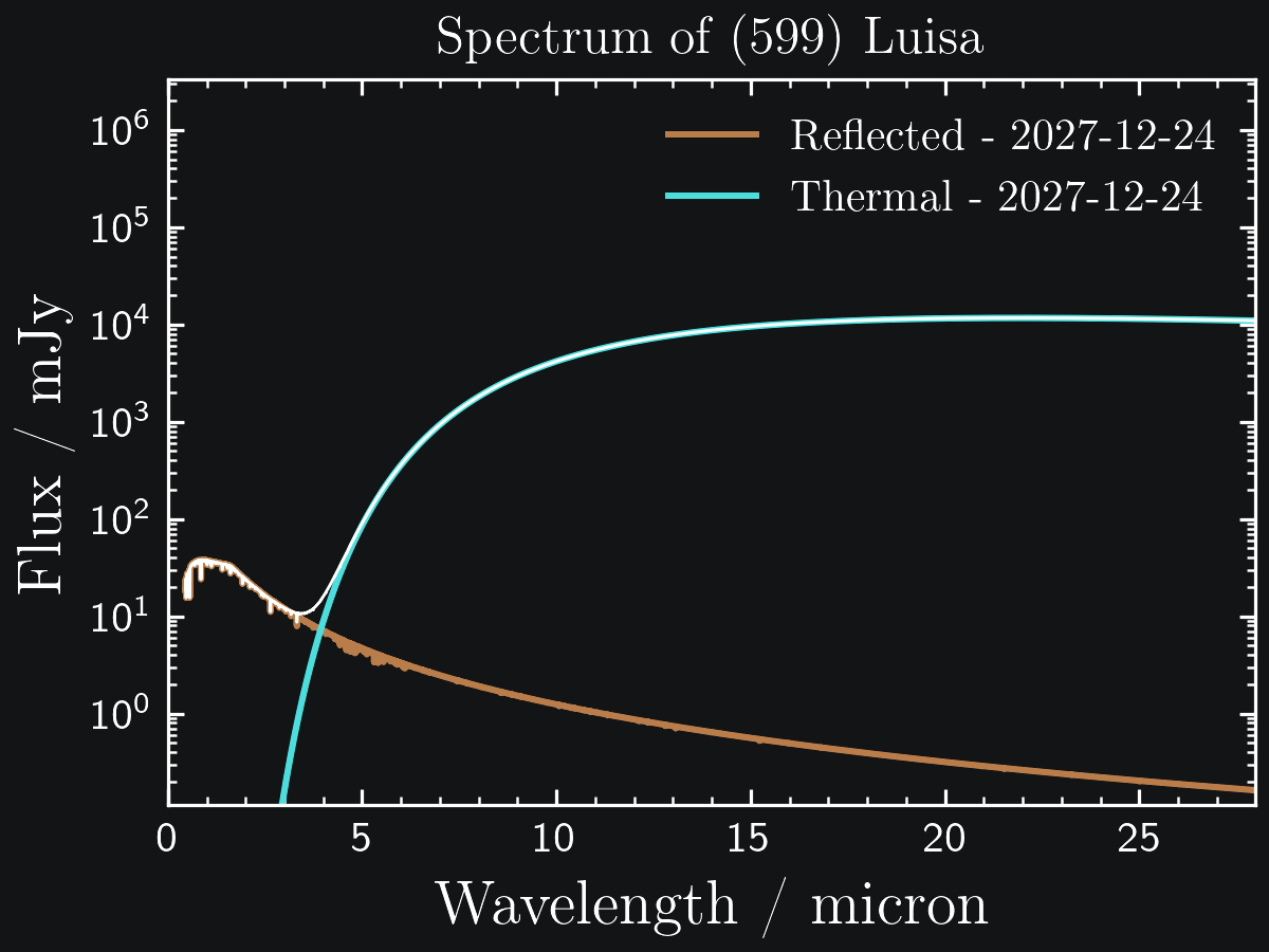
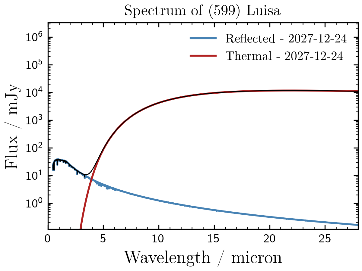
^{Fig. 1: (599) Luisa on 2027-12-24.}

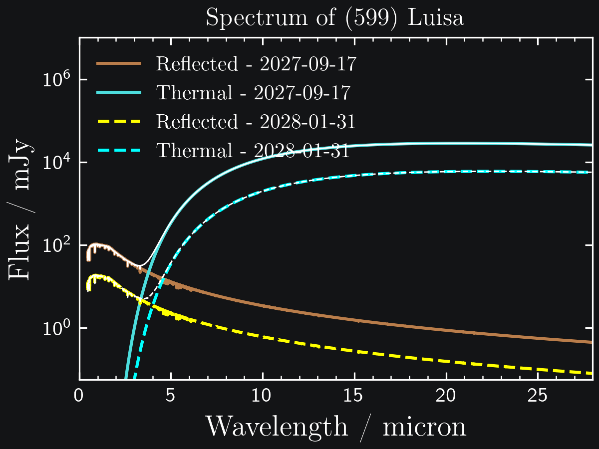
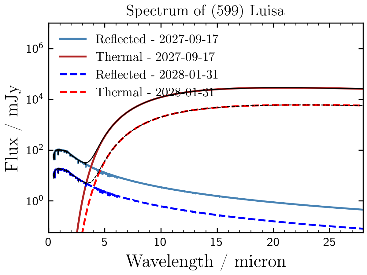
^{Fig. 2: (599) Luisa at highest and lowest thermal flux.}